Introduction

Defining Computational Science

Before embarking on our journey to learning how computational science is used to solve scientific and engineering problems, we should first establish more formally what we mean by computational science. When you think of the word “computation,” what comes to mind? Perhaps you recall practicing long division in elementary school, balancing your checkbook, or estimating groceries required for a dinner party. These are instances of equating computation to arithmetic, but the modern conception of computation in science and engineering goes well beyond this concept.

We will begin our overview of computational science by defining it and showing the breadth of disciplines and enterprises that make use of it to solve problems. Computational science sounds a lot like computer science, but it is a different discipline, although it does involve computer science. Here is a good working definition that we will use:

Computational science is the development or application of techniques that use computation to solve scientific and engineering problems.

There are certainly other definitions that can be found in the literature, but this definition will work for us.

Computational science is inherently interdisciplinary, involving concepts and techniques from computer science, mathematics, and a domain-specific science or engineering discipline.

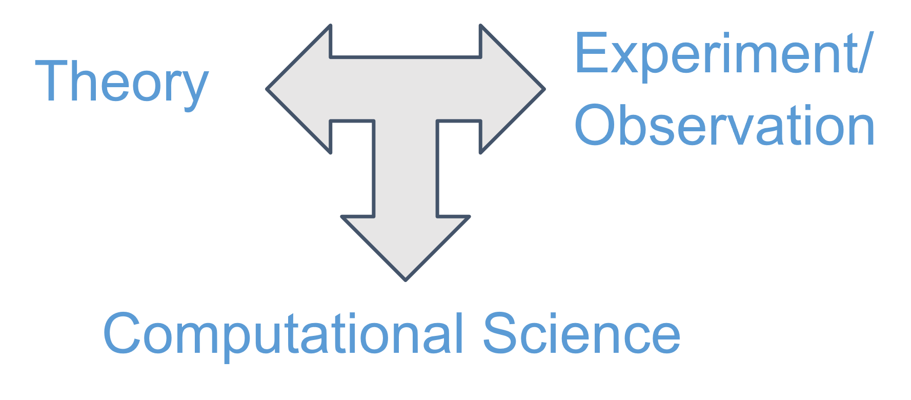
Traditionally, a scientific discipline involves two reinforcing ways of working: experiment (or observation) and theory. Figure 1 illustrates these two essential aspects of science.

Figure 1: Traditional concept of science.

The existence of powerful computing technologies has changed the conduct of scientific and engineering work profoundly by allowing large data sets to be studied and realistic models of systems to be simulated. Computation aids both theoretical and experimental work, so that computational science becomes an indispensable third leg of our concept of scientific work, as illustrated in Figure 2.

Figure 2: The modern concept of science.

Consider the scientific discipline astronomy. Current observational techniques have created huge amounts of data that include objects located (stars, galaxies, exoplanets, etc.), motion data of each object, intensity of electromagnetic radiation at different wavelengths associated with these objects, and other properties. Table 1 shows the amount of data generated by several observational projects. Note that TB stands for terabyte (10¹²), PB stands for petabyte (10¹⁵), and EB stands for exabyte (10¹⁸). We see that each of these individual projects creates enormous amounts of data.

Table 1: Data volumes of different sky survey projects (Zhang & Zhao, 2015).

Sky Survey Projects	Data Volume
DPOSS (The Palomar Digital Sky Survey)	3 TB
2MASS (The Two Micron All-Sky Survey)	10 TB
GBT (Green Bank Telescope)	20 PB
GALEX (The Galaxy Evolution Explorer )	30 TB
SDSS (The Sloan Digital Sky Survey)	40 TB
SkyMapper Southern Sky Survey	500 TB
LSST (The Large Synoptic Survey Telescope)	\(\sim\)200 PB expected
SKA (The Square Kilometer Array)	\(\sim\)4.6 EB expected

Cataloging, storing, uncovering systematic errors, and performing exploratory data analysis all require significant computational resources and specialized techniques.

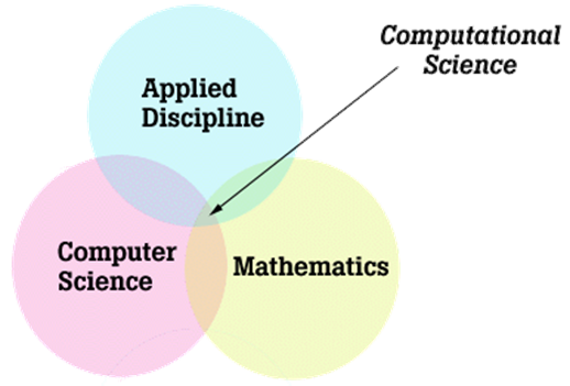
Another way to think of computational science is that it involves the intersection between computer science, mathematics, and an applied discipline, as illustrated in Figure 3.

Figure 3: Conceptual model of computational science (The Shodor Education Foundation, 2000) .

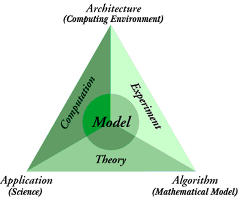
Mathematical modeling is a central activity for working physicists and engineers. As other sciences have become more quantitative, mathematical modeling has assumed an increasingly important role in those disciplines as well. This includes areas such as biology and environmental sciences. A significant amount of work in contemporary computational science involves developing and exploring mathematical models using computation. This focus will be important to us throughout this course, so it is worth keeping in mind how modeling connects with other aspects of doing science. Figure 4 illustrates the connections.

A model starts with experimental data or observations and describes patterns in the data, connecting those patterns with more fundamental theoretical ideas from the area of science being investigated. The process of uncovering patterns typically involves elements of computation such as statistical analysis and visualizations. The outer elements of Figure 4 illustrate key elements of computational science itself: a scientific activity (application) that is facilitated by using mathematics and algorithmic thinking (algorithms), which, in turn, requires computation to fully explore (computing environment).

Figure 4: The relationships between models, the basic elements of science, and elements of computational science (The Shodor Education Foundation, 2000).

Examples of Computational Science Applications

Let’s look at some specific examples of scientific and engineering problems that use computation science.

Global Climate Change

Climate change is an important topic that impacts many areas of everyday life and promises to have even more profound effects in the future. It is important for us to understand how to describe climate, recognize the important determinants of climate, and develop realistic models that can help us predict the future climate.

Describing the global climate starts with some basic observational data such as the average surface temperature. Figure 5 shows data on the average surface temperature. Notice that the graph does not directly show the temperature, but rather the temperature anomaly, which is the difference between the actual temperature and the average temperature measured over a specified base time period. Using the temperature anomaly avoids including effects of systematic errors in an individual thermometer.

Figure 5: Average surface temperature anomaly (Temperature Composite, n.d.).

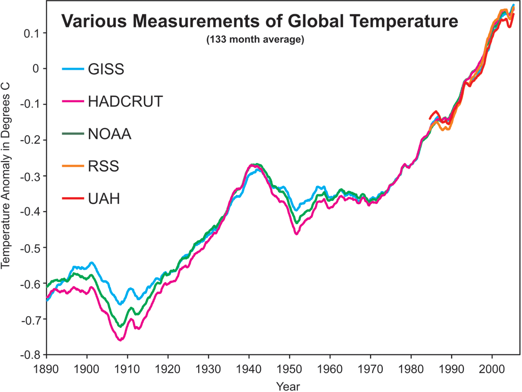
Producing just this one graph involved many aspects of computational science.

• The individual data sets contain a large number of measurements that must be made available in a user-friendly form.

• Each data set must undergo statistical analysis to uncover and correct for problems in the data.

• A moving average is calculated to remove some of the random variation present in the observations. Such smoothing of the data helps to identify trends

• The graph of the moving average must be generated.

Each of these actions requires computation to accomplish.

The graph helps us to identify patterns, namely, that average global surface temperature increased from 1910 to 1940, leveled off and decreased slightly between 1940 and 1950, then increased again at a faster rate from 1950 to the present.

Another way of visualizing the data that requires significant computational work is to show the temperature anomaly in different regions of the earth and follow the geographic distribution over time. Figure 6 shows the result of performing this kind of analysis. The level of the temperature anomaly is indicated by the intensity of the color.

Figure 6: Geographic distribution of the temperature anomaly (NASA’s Scientific Visualization Studio, 2021).

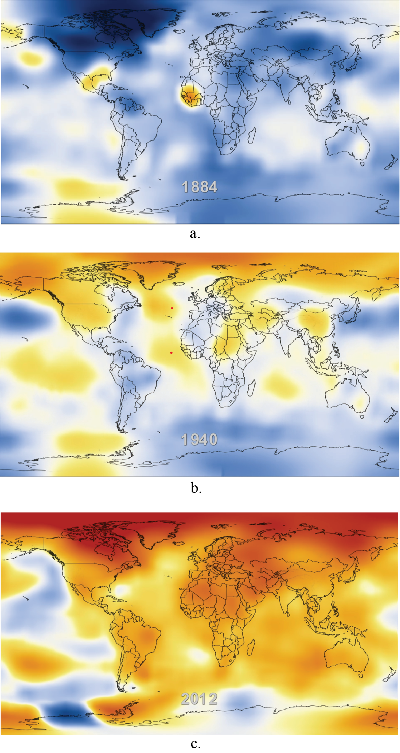
Creating visualizations of the temperature data is only the beginning of investigating climate change. Models based on fundamental science including physics, chemistry, and meteorology must be constructed to help us understand the underlying causes for the changes we see. These models typically are mathematically sophisticated and can usually only be explored using numerical calculations performed by a computer.

Evolution of Cosmic Structures

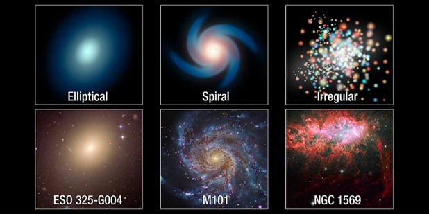
Understanding how specific cosmic structures, such as galaxies, evolve over the history of the universe is an important problem of current interest. Observational astronomers can locate and characterize galaxies that have existed since a few million years after the Big Bang. Figure 7 shows some of the different kinds of galaxies found in the universe. Progress in understanding how the observed distribution of galaxy morphologies has recently been made by using computer simulations based on fundamental astrophysics principles incorporating hydrodynamics and gravitation principles (Vogelsberger et al., 2014). The researchers began with a system approximating the state of the universe at 12 million years after the Big Bang.

Figure 7: Three general galaxy morphologies with specific examples of each. (Feild, 2019).

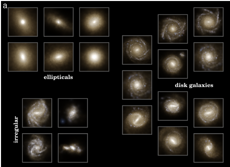
The computer simulation over about 13 billion years of evolution was able to show realistic distributions of galaxy morphologies. Figure 8 shows some of the simulated galaxies produced from the simulation.

Figure 8: Simulated galaxy morphologies produce by computer simulation of galactic structure evolution (Vogelsberger et al., 2014).

Designing the Boeing 777

The Boeing 777, shown in Figure 9, is a twin-engine, wide-body, commercial jet that was first introduced in 1994 but is still in production.

Figure 9: . The Boeing 777 commercial jet (Koske, 18 October 2009, 11:52).

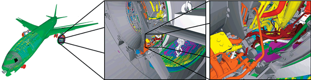
It was a significant achievement of engineering because it was the first airplane to be completely designed using computer-assisted design tools (CAD). This eliminated the need for most full-scale mock-ups. This reduced the time and cost of designing and revising all the systems involved in the aircraft. The CAD system combined significant engineering mechanics knowledge with extremely sophisticated computer graphics to ensure that all parts of the system fit to within required tolerances and could move correctly. The CAD system also had properties of the materials used for parts built in so that stresses and strains could be measured in the simulated system to ensure part failure would not occur. Each system of the plane could be simulated through multiple cycles of revisions with both software and human-based visual checks. Figure 10 shows examples of the visual product from the CAD system.

Figure 10: Graphics output from the CAD software used for designing the Boeing 777 (Dietrich et al., 2005).

Every major area of science and engineering now has an established subarea that is focused on developing appropriate computational approaches to problem-solving in the particular discipline. The following is a list of such disciplines:

• Computational Biology

• Computational Chemistry

• Computational Economics

• Computational Finance

• Computational Neuroscience

• Computational Physics

• Computational Sociology

Elements of Computational Thinking

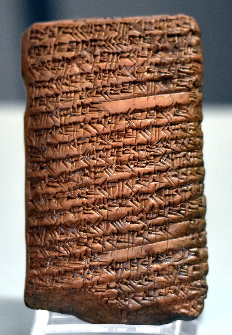
While the term “computational thinking” is relatively new, having been popularized in 2006 by Jeannette Wing in an opinion piece about computer science education (Wing, 2006), but concepts associated with the term have a long history. The ancient Babylonians (1800-1600 BCE) developed tables of reciprocals and multiplications to speed up and systematize arithmetical calculations. They also developed step-by-step procedures (i.e., algorithms) for solving certain classes of algebra problems (Knuth, 1972). Figure 11 shows an example of a Babylonian clay tablet specifying the procedure for solving a mathematical problem (Amin, 14 March 2019, 11:03:07).

Historical Examples of Computational Thinking

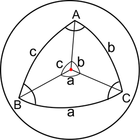
The Ancient Greek astronomer Hipparchus (190-120 BCE), shown in Figure 12, developed a theoretical framework to predict positions of sun and moon as functions of time. This framework used relationships from spherical trigonometry, and the required calculations used regular trigonometric functions such as cosine and sine. To expedite calculations involving trig functions, Hipparchus developed procedures for producing trigonometric function tables. Such tables remained useful well into the 20^th century before being replaced by electronic calculators.

Figure 11: Babylonian clay tablet describing a mathematical procedure (Amin, 14 March 2019, 11:03:07).

Figure 12: he Greek astronomer Hipparchus (New York Public Library / Science Source / Science Photo Library, n.d.).

An example of a spherical triangle is shown in Figure 13.

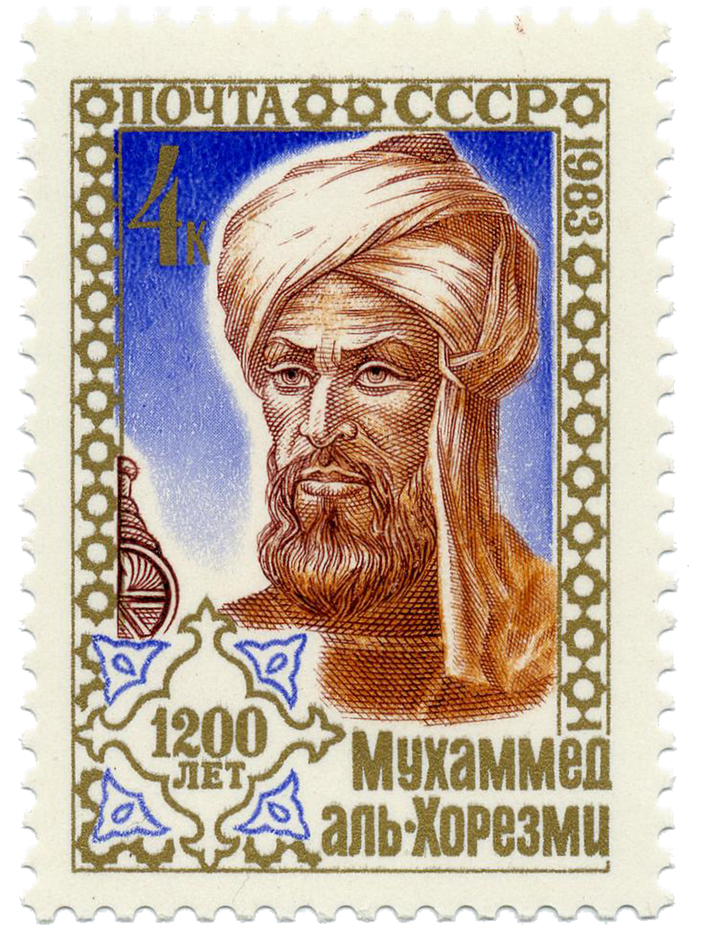
The Persian mathematician Muhammad ibn Musa al-Khwarizmi, shown in Figure 14, wrote an important book published around 800 CE that specified procedures for solving quadratic equations. The Latin translation of his book on the Hindu-Arabic numeral system, Algoritmi de numero Indorum, gave us the term “algorithm”, which will play a significant role in our overview of computational thinking.

Figure 13: Example of triangle on a sphere (Mercator, 2013).

Figure 14: Commemorative Stamp of Muḥammad ibn Mūsā al-Ḵwārizmī (unknown, 1983).

There is not a universal definition for the term “computational thinking”, yet it is really central to your development as a computational scientist. So, how can you be expected to learn how to do something so important when it cannot be defined?  Life is truly unfair. But do not despair; we will look at some elements of computational thinking that most computational scientists will agree are important elements of learning how to approach problems so that they can be solved computationally.  Indeed this can be a starting point for our working definition of computational thinking. Here is how Jeannette Wing of Columbia University defines it:

Computational thinking is the thought processes involved in formulating a problem and expressing its solution(s) in such a way that a computer—human or machine—can effectively carry it out (Wing, 2014).

An athlete must train their body to execute physical motions required by the sport.  A computational scientist must train their mind to think about problems in a way that allows computers to help solve the problems.  Computational thinking is not used only for solving problems with a computer but can provide strategies for solving all sorts of problems.  The habits of mind and processes you will learn here can be widely applied.

Uses of Computational Thinking

Computational thinking is used in many disciplines and activities with significant real-world applications:

• Mapping the human genome

• Predicting the spread of infectious disease

• Developing methods for weather prediction

• Predicting the effect of government policies

• Developing a method of scheduling meetings efficiently in a large organization

Pillars of Computational Thinking

The general principles of computational thinking can be represented using four pillars, or principle concepts. They are

• Decomposition

• Pattern Recognition

• Data Representation and Abstraction (we can shorten this to just Abstraction)

• Algorithms

Let’s consider each of these pillars.

Decomposition involves breaking a complex problem into smaller, more-manageable sub-problems or parts. Consider the problem of writing a paper for a course. We might break this problem into at least three parts: writing an introduction, writing the main body, and finally writing a conclusion.

Activity: Consider the problem of cleaning your apartment or house. Apply the process of decomposition to this problem.

Pattern recognition involves finding similarities or shared characteristics within or between problems. If two problems share characteristics, then the same solution can be used to solve both problems.

Activity: Think of a problem for which you could use computational thinking, describe it, and then describe how you would apply pattern recognition.

The third pillar of computational thinking is called data representation and abstraction. We will shorten this to just abstraction. The key element of abstraction is to determine the characteristics of a problem that are important and those that can be ignored. Next, we decide on a way to represent the chosen important characteristics. This would be the data representation.

Example: developing an online book catalog. Important information:

• Title

• Authors

• ISBN

• Year of publication

• Edition

Unimportant information:

• Book jacket color

• Author birthplace

Activity: Think of a problem for which you could use computational thinking, describe it, and then describe how you would apply data representation and abstraction.

The final pillar of computational thinking is algorithms. We will explore algorithms throughout this course. For now, we define their essential properties as:

1. A collection of individual steps to be used in solving the problem;

2. Each step must be defined precisely;

3. The steps must be performed sequentially.

We can represent an algorithm using a flow chart.

The elements of flowcharts include

1. Terminals: an oval that represents a start or stop.

   

2. Input/Output: a parallelogram that represents the program either getting data input or creating data output.

   

3. Processing: a box that represents executing some action such as performing arithmetic.

   

4. Decision: a diamond represents making a decision.

   

5. Flow Lines: arrows that indicate the sequence taken by instruction. The arrows are called directed edges by computer scientists.

   

Another way of representing an algorithm is using pseudocode, which we will explore later.

Logical Arguments

A good starting point for computational thinking is the idea of logical thinking. Logic is a systematic approach to distinguish between incorrect and correct arguments. Logical reasoning starts with premises, which are statements about initial knowns concerning the problem.  Premises must be determined to be true or false. If the premises are true then the final step in a logical argument is to reason that a conclusion follows.  

There are two general categories of logical arguments with which we are concerned: deductive and inductive arguments. In a deductive argument, once the premises are established to be true then the conclusion will necessarily follow with complete certainty.  In an inductive argument the veracity of statements, whether they be premises or a conclusion, can be expressed only with a particular probability rather than with certainty.

Example of deductive reasoning:

1. Socrates is a man.

2. All men are mortal.

3. Therefore, Socrates is mortal

Statements 1 and 2 are the premises.  If they are both true then the conclusion necessarily follows.  

A deductive argument can fail in two ways:

1. One or more of the premises could be false, which means that the conclusion is not necessarily true.

2. The conclusion does not necessarily follow from the premises, even if they are all true.  There is a logic problem in the argument.

Example of inductive reasoning:

In an inductive argument there will be an element of probability involved in the truth of premises and conclusion.  In an inductive argument we establish that the conclusion is probably true but we cannot say it is true with certainty, as we can with a deductive argument.  Here is an example:

• 90% of the senior class at Belmont High were accepted into college.

• Robert is a senior at Belmont High

• Therefore, Robert was accepted into college.

The conclusion is probably true but not necessarily true.

Computers most easily perform deductive reasoning.  In the next Module, we will learn about a particular way of performing deductive arguments called Boolean logic that is implemented in all programming languages, including Python.

Mathematical Modeling in Science and Engineering

Modeling is a fundamental element of science and engineering. We can think of a model as a simplified representation of a system of interest. A model could be physical such as letting a basketball represent the sun and a golf ball represent the earth and carry the golf ball around the basketball to illustrate a planetary orbit. Automobile manufacturers historically used clay models of a vehicle to explore how the shape influenced airflow around the vehicle. In science and engineering models are usually represented using mathematics such as representing the position of a planet by its spatial coordinates \((r,\theta,\phi)\) in a spherical coordinate system and then representing the orbit by the equation for an ellipse, Equation 1

\[ r = \frac{a\left(1- e^2\right)}{1 + e\cos \left(\phi \right)} \tag{1}\]

We can usefully classify the kinds of models used in science and engineering into the following categories.

• Deterministic

• Stochastic

• Empirical

• Theory-based

Deterministic Models

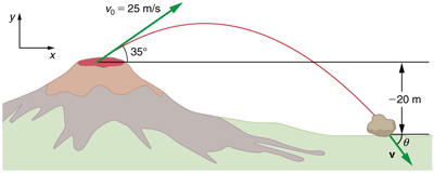
Deterministic models describe systems in which knowledge of the state at one time will determine the state at subsequent times. There is no element of randomness in the state of the system. An example would be applying Newton’s laws of motion to a rock thrown in the air. Knowing the rock’s position and velocity at one time will allow us to predict the position and velocity at subsequent times. Figure 15 illustrates this situation.

Figure 15: Trajectory of a rock ejected from a volcano. (Paul Peter Urone & Roger Hinrichs, 2012)

Stochastic Models

Stochastic models involve some element of randomness. When such models are described mathematically, they will involve use of probability theory. An example is modeling the trajectory of smoke coming from a burning candle, as shown in Figure 16. The first part of the smoke trajectory after it leaves the wick could be described using a deterministic model, but most of the smoke motion involves an element of randomness, suggesting that a stochastic model would be required.

Figure 16: Candle smoke (Wicks, 2022)

Empirical Models

Empirical models attempt to find the mathematical form relating variables used to describe raw observational data or experimental results. The model is purely descriptive and not interpreted as an explanation of a pattern based on more fundamental principles. For example, suppose we take stroboscopic photographs of a falling ball at equal time intervals, as shown in the photo of Figure 17. If we measure the ball’s position as a function of time from the photograph and make a graph, we will obtain the graph in Figure 17.

Figure 17: (a) Stroboscopic photographs of a falling ball (Maggs, 2007). (b) Graph of position data.

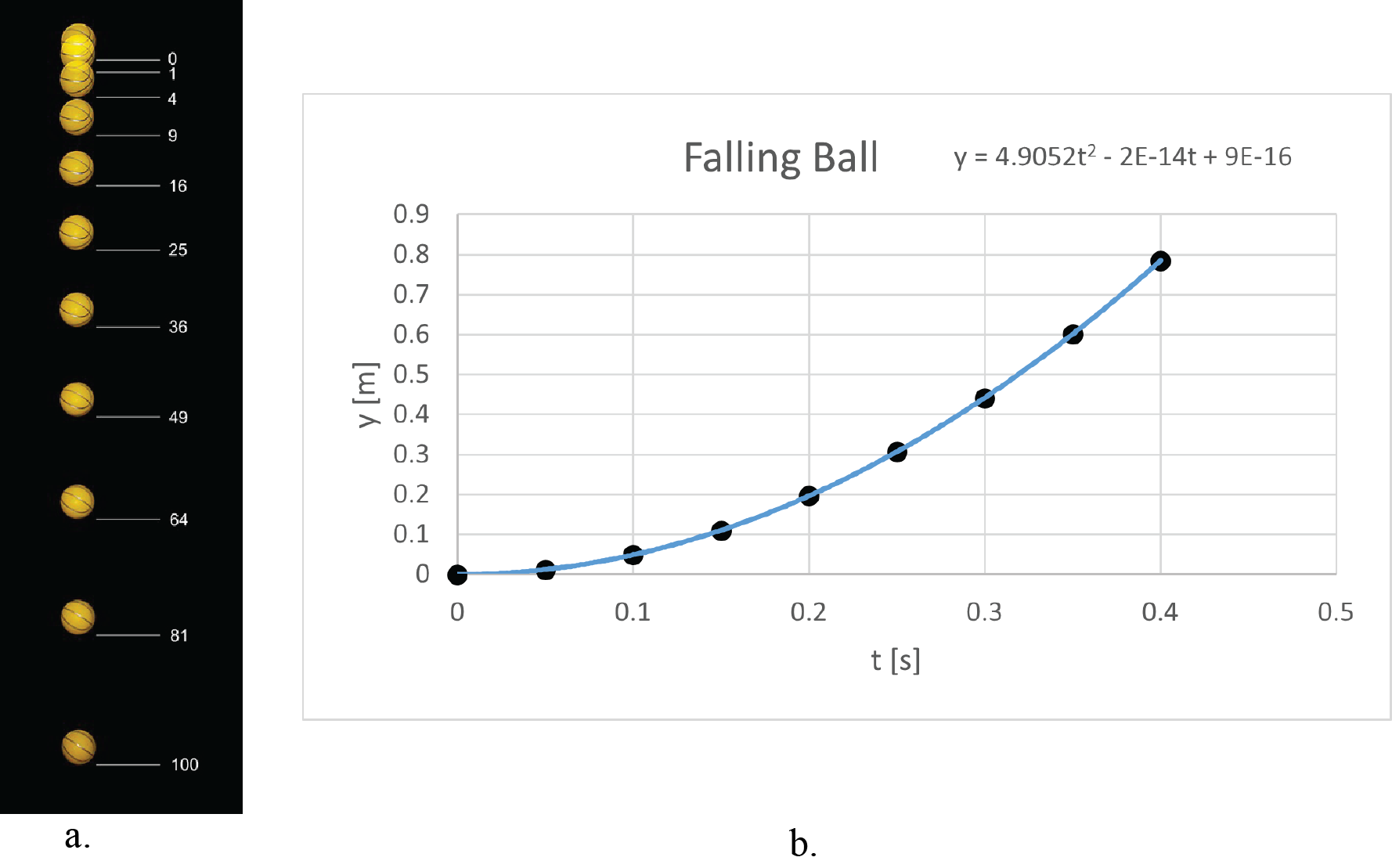
Looking at the graph of the position data taken from strobe photos, we would rule out a linear relationship between y and t. The next type of equation to try would probably be a second-order polynomial, a quadratic. Such a model does fit the data well, as shown by the solid line in the graph.

Theory-based Models

Theory-based models use the more fundamental elements of a scientific theory, such as Newton’s Laws of Motion in physics, to develop the mathematical model of a system. In the example of the dropped ball, described above, we can apply Newton’s Second Law and Newton’s Law of Gravitation to the ball and predict that that relationship between the ball’s position and time should be a second-order polynomial equation, assuming that we ignore the effects of air resistance. We would arrive at the same equation as we hypothesized just on the basis of looking at the data, but the equation now is seen to be implied by the theory called Newton’s Laws of Motion.

The categories described above are not exclusive of each other. We can have theory-based deterministic models or theory-based stochastic models, for example.

We will use a variation on our four-step problem-solving strategy discussed in Chapter 2 when developing a mathematical model of a system. Here are the basic steps.

1. Analyze the problem

2. Formulate a model

3. Solve the model

4. Verify and interpret the model’s solution

5. Report on the model

6. Maintain the model

Our discussion of dynamical systems models will illustrate the use of this strategy.

Introduction to Textbook Computing Environment

Many principles of computational science are independent of the programming language used to implement the computations, but it is easier to learn these principles using specific examples that involve a particular programming language. We will use Python as our primary programming language. To enable quick development and application of computational science principles we should establish a working Python programming environment now, so that it can be used immediately.

Types of Programming Environments

There are several ways to establish a good programming environment that uses Python:

1. We can download and install a Python distribution, such as the Anaconda Distribution and then use the IPython command line shell that comes with that distribution. This allows the user to execute Python interactively, one code line at a time.Install a Python distribution, such as Anaconda, that comes with a Jupyter server then use Jupyter notebooks to compose executable code and text blocks.

2. Install a Python distribution, such as Anaconda, then use a plain text editor (notepad, gedit, TextEdit) application to compose code and then execute the code from the command line using the appropriate command line console for your operating system.

3. Install a Python distribution, then install an IDE application (PyCharm, Spyder, VSCode) that bundle a smart text editor, an interactive console, and enhanced debugging tools into a nice GUI.

4. Use a cloud computing platform such as CoCalc, pythonanywhere, or Google Colab that allows the user to use Jupyter notebooks without installing any software, except for a browser. The cloud service maintains the Python distribution.

The Google Colab Environment

The last method is easiest and quickest to use, so we will focus on it here. The other methods are discussed in the appendix. We will use Google Colab for our example. To use Jupyter notebooks in Colab do the following.

1. Sign into your Google account.

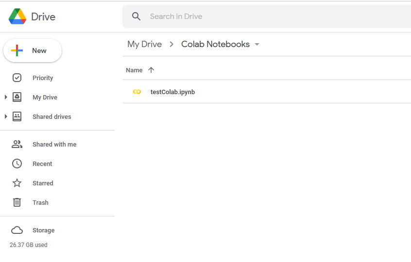
2. Go to your Google Drive and create a folder that will contain your Colab notebooks, which will be named Colab Notebooks. Open the folder that you just created.

3. Open a new browser tab and goto https://colab.research.google.com. You will see the following window showing available file spaces:

Initial Google Colab window.

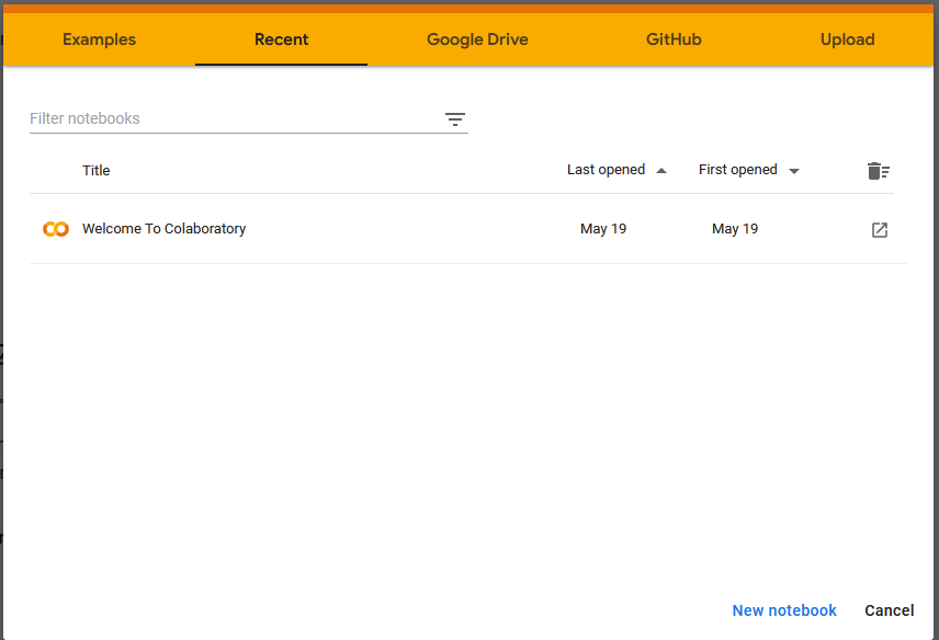
1. Select the examples tab and select the Overview of Colaboratory Features notebook.

2. Read through this notebook to get oriented to the Colab Jupyter notebook features.

Note that there are two kinds of cells in the notebook: text cells and code cells. Code cells contain executable Python code. The cell contents can be executed by selecting the Play icon on the left of the cell or by clicking anywhere in the cell and typing Shift+Enter.

Let’s now create a new Colab notebook from your Google Drive folder.

Navigate to your Colab notebook folder that you created previously:

Figure 18: Initial Google Colab window.

Select

• + New

• More

• Google Colaboratory

Figure 19

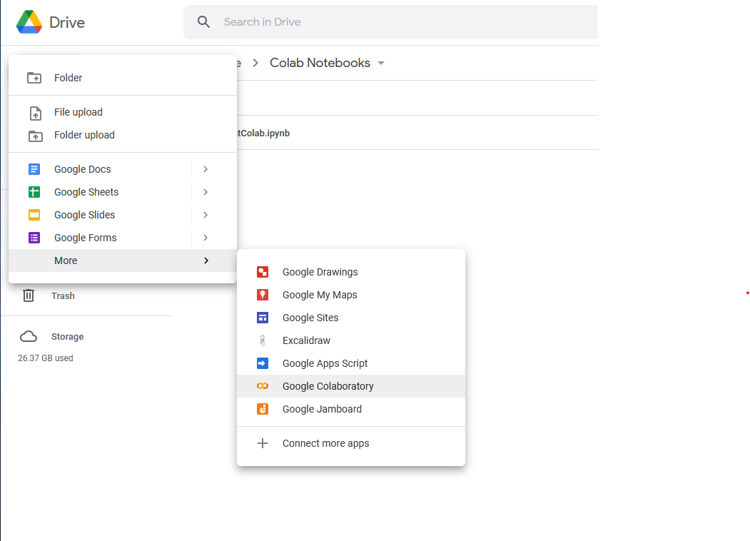
You will get a new Colab Jupyter notebook in your folder, as shown in Figure Figure 20.

Figure 20: New Colab notebook.

The new notebook is named Untitled0.ipynb by default. You can change the name as you would any Google Doc file. Leave the ipynb extension since that indicates that the file is a Jupyter notebook file.

The new notebook starts with one code cell. It is good practice to include documentation in your notebook, so let us put a text cell above the first code cell.

Place the mouse pointer right above the code cell so that the add code or text buttons appear.

Choose the + Text option.

Figure 21

A text cell will appear above the code cell. Double click in the cell to begin text editing.

You should see an editing box on the left and a preview of the rendered text on the right.

Figure 22

You can provide formatting of the text using Markdown syntax. The example below shows how to create a heading. We will discuss Markdown syntax later.

Figure 23

After you finish entering any text then click the Close Markdown icon (circled above).

When you create a Colab notebook you can easily save the file in your Google Drive by selecting

File > Save

Colab will also create a temporary folder accessible to the notebook while it is open. You can view the contents of this folder by selecting the File Explorer tool on the left.

Figure 24

This folder will disappear when the notebook file is closed, so if your code writes to a file you will want to ensure that the file gets placed where it will not be lost. One way to do this is to connect your Google Drive to the Colab notebook while it is running. This can be done using the Mount Google Drive tool.

Figure 25

You will now see your Google Drive as a folder in the File Explorer area.

Figure 26

Later, we will learn how to write directly to a file in the MyDrive folder using Python code in the notebook.

Exercises

1. Choose an area of science or engineering that interests you. Table 2 below lists areas that have a well-established record of computational solutions. Perform a web-based search using Google and library search resources to find a specific problem in the area that required computation to solve. Create a bibliography of these sources.

Table 2: Wikipedia pages for areas of computational science.

Computational archaeology	Computational mathematics
Computational astrophysics	Computational mechanics
Computational biology	Computational neuroscience
Computational chemistry	Computational particle physics
Computational materials science	Computational physics
Computational economics	Computational sociology
Computational electromagnetics	Computational statistics
Computational engineering	Computational sustainability
Computational finance	Computer algebra
Computational fluid dynamics	Financial modeling
Computational forensics	Geographic information system (GIS)
Computational geophysics	High-performance computing
Computational history	Machine learning
Computational informatics	Network analysis
Computational intelligence	Neuroinformatics
Computational law	Numerical weather prediction
Computational linguistics

You should create a document that includes the following:

• A paragraph that describes the problem.

• A paragraph that describes why computation was required for solving or investigating the problem.

• Four (or more) references that give information on the problem. At least two of the references should be peer-reviewed sources such as research journal papers and academic books.

2. Computational science can be thought of as the intersection between a scientific or engineering discipline such as biology, mathematics, and _______________________ .

3. Computer science is the study of algorithms whereas computational science is the study of how _____________________ can be used to solve scientific problems.

4. Traditional science would study a system by experimenting with the actual system and developing theories to help understand the system. Computational science adds to this approach by using _____________ to analyze and visualize data and to explore properties of mathematical _____.

5. Which of the following are considered pillars of Computational Thinking, as defined in this course? (Choose all that are true.)

1. algorithms
2. arithmatic
3. Python
4. abstraction
5. decomposition
6. applied science
7. pattern recognition

6. Algorithms can be represented using

1. flowcharts
2. graphs
3. equations
4. mathematical variables

7. Select the statements below that are true concerning deductive reasoning.

1. The conclusion is probably rather than certain.
2. The conclusion necessarily follows from the premises.
3. An argument could be valid but unsound.

References

Amin, O. S. M. (2019). Babylonian Clay Tablet [Photograph]. Own work. https://commons.wikimedia.org/wiki/File:Clay_tablet,_mathematical,_geometric-algebraic,_similar_to_the_Pythagorean_theorem._From_Tell_al-Dhabba%27i,_Iraq._2003-1595_BCE._Iraq_Museum.jpg

Dietrich, A., Wald, I., & Slusallek, P. (2005). Large-scale CAD Model Visualization on a Scalable Shared-memory Architecture. In G. Greiner, J. Hornegger, H. Niemann, & M. Stamminger (Eds.), Vision, Modeling, and Visualization 2005 (pp. 303–310). Akademische Verlagsgesellschaft Aka.

Feild, A. (2019). Galaxy Types. https://hubblesite.org/contents/media/images/4508-Image.html

Knuth, D. E. (1972). Ancient Babylonian algorithms. Communications of the ACM, 15(7), 671–677. https://doi.org/10.1145/361454.361514

Koske, K. (2009). United Airlines B777-222 N780UA. United Airlines Boeing 777-222 (N780UA) Uploaded by Altair78. https://commons.wikimedia.org/wiki/File:United_Airlines_B777-222_N780UA.jpg

Maggs, M. (2007). Falling Ball [Digital]. https://commons.wikimedia.org/wiki/File:Falling_ball.jpg

Mercator, P. (2013). Spherical trigonometry [Digital]. https://commons.wikimedia.org/wiki/File:Spherical_trigonometry_basic_triangle.svg

NASA’s Scientific Visualization Studio. (2021, January 14). SVS: Global Temperature Anomalies from 1880 to 2020. NASA Scientific Visualizations Studio. https://svs.gsfc.nasa.gov/4882

New York Public Library / Science Source / Science Photo Library. (n.d.). Hipparchus, Greek Astronomer and Mathematician [Digital]. https://www.sciencephoto.com/media/1011097/view

Temperature Composite. (n.d.). Skeptical Science. Retrieved January 9, 2022, from https://skepticalscience.com//graphics.php?g=7

The Shodor Education Foundation. (2000). Overview of Computational Science. ChemViz Curriculum Support Resources. http://www.shodor.org/chemviz/overview/compsci.html

unknown. (1983). Commemorative Stamp of Muḥammad ibn Mūsā al-Ḵwārizmī. https://commons.wikimedia.org/wiki/File:1983_CPA_5426_(1).png

Urone, P. P., & Hinrichs, R. (2012). 3.4 Projectile Motion. In College Physics. OpenStax.

Vogelsberger, M., Genel, S., Springel, V., Torrey, P., Sijacki, D., Xu, D., Snyder, G., Bird, S., Nelson, D., & Hernquist, L. (2014). Properties of galaxies reproduced by a hydrodynamic simulation. Nature, 509(7499), 177–182. https://doi.org/10.1038/nature13316

Wicks, R. (2022). Twelfth night [Digital]. https://unsplash.com/photos/FMARk9s_20s

Wing, J. M. (2006). Computational thinking. Communications of the ACM, 49(3), 33–35. https://doi.org/10.1145/1118178.1118215

Wing, J. M. (2014, January 10). Computational Thinking Benefits Society. Social Issues in Computing. http://socialissues.cs.toronto.edu/index.html%3Fp=279.html

Zhang, Y., & Zhao, Y. (2015). Astronomy in the Big Data Era. Data Science Journal, 14(0), 11. https://doi.org/10.5334/dsj-2015-011

Amin, O. S. M. (14 March 2019, 11:03:07). Babylonian Clay Tablet [Graphic]. https://commons.wikimedia.org/wiki/File:Clay_tablet,_mathematical,_geometric-algebraic,_similar_to_the_Pythagorean_theorem._From_Tell_al-Dhabba%27i,_Iraq._2003-1595_BCE._Iraq_Museum.jpg

Dietrich, A., Wald, I., & Slusallek, P. (2005). Large-scale CAD Model Visualization on a Scalable Shared-memory Architecture. In G. Greiner, J. Hornegger, H. Niemann, & M. Stamminger (Eds.), Vision, Modeling, and Visualization 2005 (pp. 303–310). Akademische Verlagsgesellschaft Aka.

Feild, A. (2019). Galaxy Types [Graphic]. https://hubblesite.org/contents/media/images/4508-Image.html

Knuth, D. E. (1972). Ancient Babylonian algorithms. Communications of the ACM, 15(7), 671–677. https://doi.org/10.1145/361454.361514

Koske, K. (18 October 2009, 11:52). United Airlines B777-222 N780UA [Graphic]. https://commons.wikimedia.org/wiki/File:United_Airlines_B777-222_N780UA.jpg

Maggs, M. (2007). Falling Ball [Graphic]. https://commons.wikimedia.org/wiki/File:Falling_ball.jpg

Mercator, P. (2013). Spherical trigonometry [Graphic]. https://commons.wikimedia.org/wiki/File:Spherical_trigonometry_basic_triangle.svg

NASA’s Scientific Visualization Studio. (2021, January 14). SVS: Global Temperature Anomalies from 1880 to 2020. NASA Scientific Visualizations Studio. https://svs.gsfc.nasa.gov/4882

New York Public Library / Science Source / Science Photo Library. (n.d.). Hipparchus, Greek Astronomer and Mathematician [Graphic]. https://www.sciencephoto.com/media/1011097/view

Paul Peter Urone, & Roger Hinrichs. (2012). Trajectory of a rock [Graphic]. https://openstax.org/books/college-physics/pages/3-4-projectile-motion

Temperature Composite. (n.d.). Skeptical Science. Retrieved January 9, 2022, from https://skepticalscience.com//graphics.php?g=7

The Shodor Education Foundation. (2000). Overview of Computational Science. ChemViz Curriculum Support Resources. http://www.shodor.org/chemviz/overview/compsci.html

unknown. (1983). Commemorative Stamp of Muḥammad ibn Mūsā al-Ḵwārizmī [Graphic]. https://commons.wikimedia.org/wiki/File:1983_CPA_5426_(1).png

Vogelsberger, M., Genel, S., Springel, V., Torrey, P., Sijacki, D., Xu, D., Snyder, G., Bird, S., Nelson, D., & Hernquist, L. (2014). Properties of galaxies reproduced by a hydrodynamic simulation. Nature, 509(7499, 7499), 177–182. https://doi.org/10.1038/nature13316

Wicks, R. (2022). Twelfth night [Graphic]. https://unsplash.com/photos/FMARk9s_20s

Wing, J. M. (2006). Computational thinking. Communications of the ACM, 49(3), 33–35. https://doi.org/10.1145/1118178.1118215

Zhang, Y., & Zhao, Y. (2015). Astronomy in the Big Data Era. Data Science Journal, 14(0, 0), 11. https://doi.org/10.5334/dsj-2015-011