Computational Thinking and Problem Solving
Dynamical Systems Modeling I
A dynamical systems model will allow a researcher to make quantitative predictions about a system, particularly with respect to the time development of important system properties. Such models are based on fundamental principles, not just empirical data, so they contribute to our basic understanding of the system being investigated. With a dynamical systems model we can make more reliable predictions about the course of a disease in a population, the metabolism of a drug in the human body, how the concentration of CO2 in the atmosphere changes over time, the motion of a space vehicle on its way to Mars, and even the motion of planets in our solar system over thousands of years.
This chapter will introduce you to some basic concepts of calculus that will make dynamical systems models easier to understand and some computational methods of solving the models to obtain predictions without having to know a lot of sophisticated mathematics.
Motivating Problem: Mathematical Model for Bacterial Growth
Pseudomonas aeruginosa is a common species of bacteria found in soil, water reservoirs polluted by animals and humans, the human gastrointestinal tract, and on human skin (Diggle & Whiteley, 2020). It is involved in opportunistic infections of people, often in hospital settings, which makes it an important microbe to study and understand. If a container of liquid growth medium is inoculated with a small sample of the microbe, then growth data such as that shown in Figure 1.1 will be obtained.
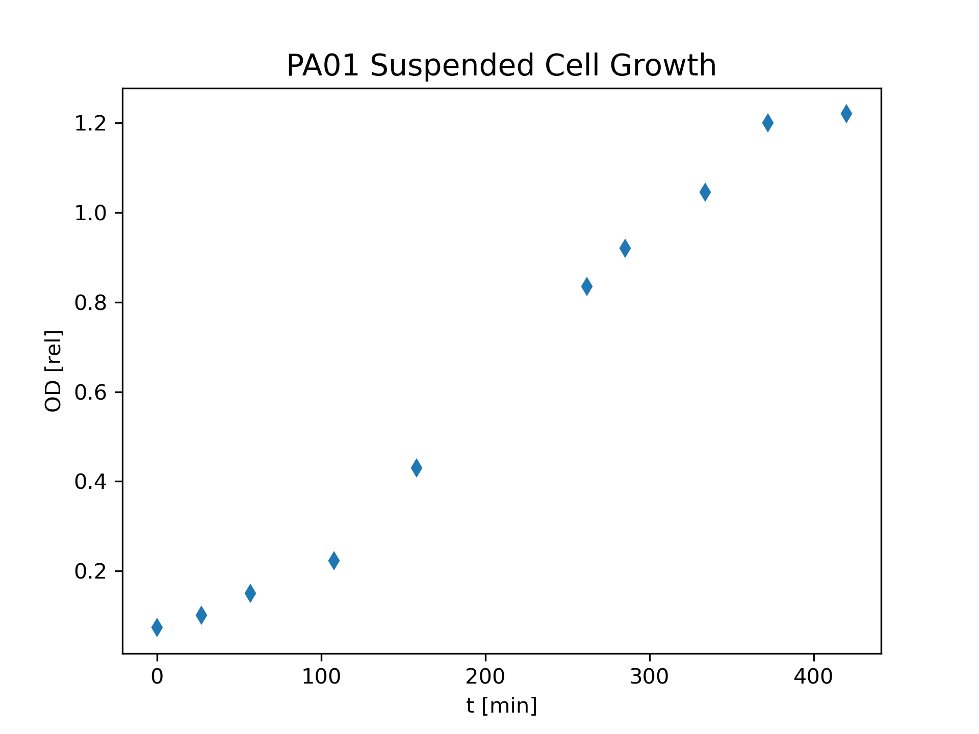
Our understanding of any microbial organism, such as Pseudomonas aeruginosa, will be aided by having an accurate mathematical model for the growth. The concepts developed in this chapter will help us to develop such a model and to simulate the model through numerical calculations done by computer.
Calculus Concepts
Your understanding of mathematical models will be aided by knowing just a couple of ideas from calculus, namely, the basic idea of a derivative of a function and the integral of a function. The goal here is not to become proficient at doing all the operations of taking derivatives or calculating integrals but to just have a basic conceptual understanding of what these mathematical things represent.
Derivatives
We will start with the derivative of a function. Consider the simple physics experiment of dropping a ball from some height and recording its position as a function of time. Table 1.1 gives some actual data taken from a video of such a ball drop. @#fig-Figure7.2 shows a graph of the data.
| t [s] | y [m] |
|---|---|
| 0.06673 | 2.693 |
| 0.1001 | 2.682 |
| 0.1335 | 2.67 |
| 0.1668 | 2.611 |
| 0.2002 | 2.576 |
| 0.2336 | 2.505 |
| 0.2669 | 2.446 |
| 0.3003 | 2.341 |
| 0.3337 | 2.235 |
| 0.367 | 2.141 |
| 0.4004 | 1.999 |
| 0.4338 | 1.882 |
| 0.4671 | 1.729 |
| 0.5005 | 1.588 |
| 0.5339 | 1.411 |
| 0.5672 | 1.247 |
| 0.6006 | 1.047 |
| 0.634 | 0.8586 |
| 0.6673 | 0.6586 |
| 0.7007 | 0.4705 |
| 0.7341 | 0.2588 |
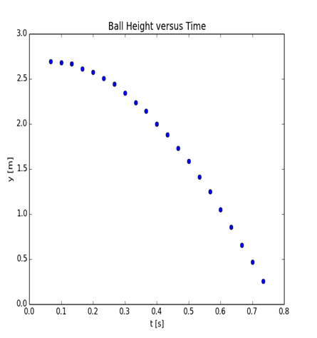
You can probably tell from the graph that the ball is speeding up over time, as it drops. The data points are at equal time intervals and the change in y clearly gets bigger as time increases. We will describe the y-coordinate by the function \(y\left(t\right)\). We define the average rate of change of \(y\left(t\right)\) by
\[\overline{v}_y = \frac{y\left(t_2\right)- y\left(t_1\right)}{t_2- t_1} = \frac{\Delta y}{\Delta t} \tag{1.1}\]
We choose to symbolize this number by \(\overline{v}_y\) because in this case it turns out to be the average velocity of the ball, hence the v. We can easily estimate the average rate of change of \(y\left(t\right)\) by using the data in the table. For the average rate of change between 0.2002 and 0.2669 [s] we have
\[\overline{v}_y = \frac{y\left(0.2669\right)- y\left(0.2002\right)}{0.2669- 0.2002} = \frac{(2.446- 2.576)\left[m\right]}{0.0667\left[s\right]} = - 1.95\left[m/ s\right] \tag{1.2}\]
The main conceptual idea of a derivative of a function such as \(y\left(t\right)\) is to calculate the average rate of change of \(y\left(t\right)\) as the time interval gets infinitesimally small. The mathematical process of doing this is taking a limit, although you do not need to worry about the details of actually doing this. We call this value the instantaneous rate of change of \(y\left(t\right)\) at a particular value of t. The symbol for the instantaneous rate of change of with \(y\left(t\right)\) respect to t at t = a is
\[\left.\frac{dy\left(t\right)}{dt}\right|_{t = a} \tag{1.3}\]
and this quantity is called the derivative of \(y\left(t\right)\) at t=a. Formally, we define
\[\left.\frac{dy\left(t\right)}{dt}\right|_{t = a} = \mathop{\text{lim}}\limits_{\Delta t\rightarrow 0}\frac{y\left(a + \Delta t\right)- y\left(a\right)}{\Delta t} \tag{1.4}\]
If you take a calculus course, you will learn a variety of techniques for performing the limit procedure. For our purposes, we can interpret the derivative geometrically. The derivative of \(y\left(t\right)\) at t = a is the slope of the tangent line to \(y\left(t\right)\) drawn at t = a. For example, Figure 1.3 shows a model calculation for the ball height \(y\left(t\right)\) with an estimate of the derivative of \(y\left(t\right)\) at t = 0.20 [s]. A straight line is drawn tangent to the curve at t = 0.20 [s], and the slope of the straight line is estimated from the rise and run. We get
\[\left.\frac{dy\left(t\right)}{dt}\right|_{t = 0.20} = \text{slope of tangent line} = \frac{- 1.69\left[m\right]}{0.80\left[s\right]} = - 2.1\left[m/ s\right] \tag{1.5}\]

Integrals
The second calculus concept we need is the integral of a function. The geometrical meaning of the definite integral of a function v(t) between t1 and t2 is the area under the curve between t=t1 and t=t2
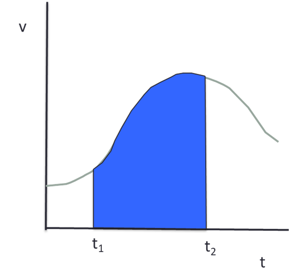
In Figure 1.4 , the shaded area represents the integral of v(t) between t1 and t2 .
Mathematicians use a special symbol to represent the integral of a function, as shown in the following equation.
\[\int\limits_{t_1}^{t_2}v\left(t\right)dt = \text{area under v-t graph from }t_1\text{ to }t_2 \tag{1.6}\]
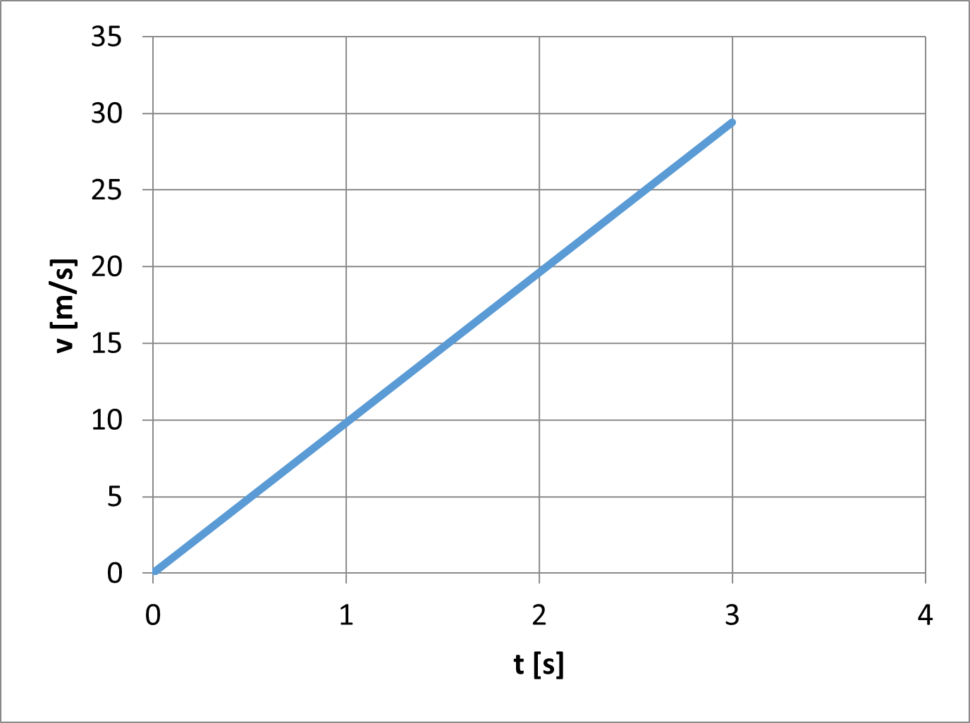
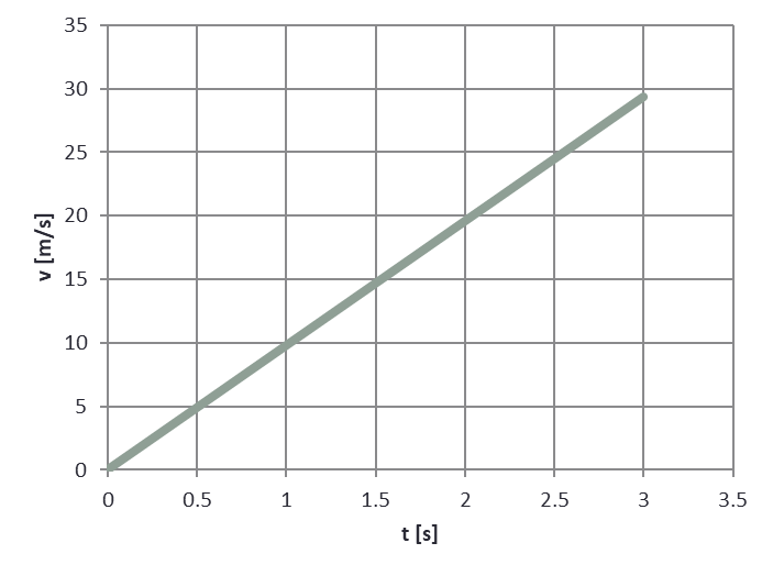
As an example, consider Figure 1.5. Let’s calculate the integral of v(t) from t = 0 to t = 2 [s].
\[\int\limits_0^2v\left(t\right)dt = \text{area under v-t graph }\text{from }\text{0[s] }\text{to }\text{2[s]}\text{=}\frac{1}{2}\text{base} \times \text{height} = \frac{1}{2} \times 2 \times 20 = 20\left[m\right] \tag{1.7}\]
The integral of a function is essentially the opposite of the derivative. In fact, if you integrate the derivative of a function you end up with the function itself. We can express this as
\[\int\limits_{t_1}^{t_2}\frac{dy}{dt}dt = y\left(t_2\right)- y\left(t_1\right) \tag{1.8}\]
Numerical Calculation of Derivatives and Integrals
Both the derivative of a function and the integral of a function can be calculated numerically with standard Python library functions. The derivative function, which we will use, is in the scipy sublibrary named differentiate (The SciPy community, 2026). A template for using the derivative function is shown below. Note that the first parameter is the function to be differentiated, and the second parameter is the value of x for which the derivative is to be calculated. The function returns a special argument that contains several pieces of information. The value of the derivative is in the float referenced by df.
import scipy.differentiate as spd
def f(x):
    return x**3
result = spd.derivative(f,2)
dfx = result.df
print(dfx)
The scipy library scipy.integrate has several functions for performing numerical integration. They differ by the algorithm used. The best first choice is the quad function (The SciPy community, 2022). Here is the basic syntax for using the quad function.
scipy.integrate.quad(f,a,b,args=())f : a Python function
a: float that is the lower limit of integral
b: float that is the upper limit of integral
args: a tuple that contains any parameters required by f
The quad function returns a tuple: (value of integral, error estimate). A template for using the quad function to perform integration is shown below.
import scipy.integrate as si
def f(t):
    return (30. - 1.8*t - 0.040*t**2)
intFunc = si.quad(f,0,5)
integral_value = intFunc[0]
Definition of A Dynamical System
A dynamical system is one that changes with time. Mathematically, it is a set of variables that describe the system of interest, and these variables will all depend on time. The state of the system is described by the value of the variables at a particular time. The present state of the system will depend on the system state in the past. The mathematical model defining the dynamical system is typically described by the state variable definitions and equations describing the rate of change for these variables.
Examples:
Population of an organism
electrical behavior of a network of neurons
Planetary positions in a stellar system
the motion of molecules in a fluid
drug concentration in a body part
many, many more biological, physical, and social systems
In the simplest case, the state of the system will be described by the value of one variable, which will be a function of time. Let us represent the state by the variable \(y\left(t\right)\), which is shown explicitly to be a function of time. y might be concentration of bacteria in a container, for example. For this one-variable system, the model is specified by the time-rate-of-change of y, which is just the derivative of y with respect to t.
\[\frac{dy}{dt} = f\left(t,y,\mathbf p\right) \tag{1.9}\]
The function f is assumed to be known. We see that it can depend on the current time t, the current value of the state variable y, and on model parameters contained in the vector p. If the value of y is known at one time, often \(t=0\), then Equation will determine the behavior of y for all subsequent t. The general term for this kind of mathematical problem is the Initial Value Problem (IVP).
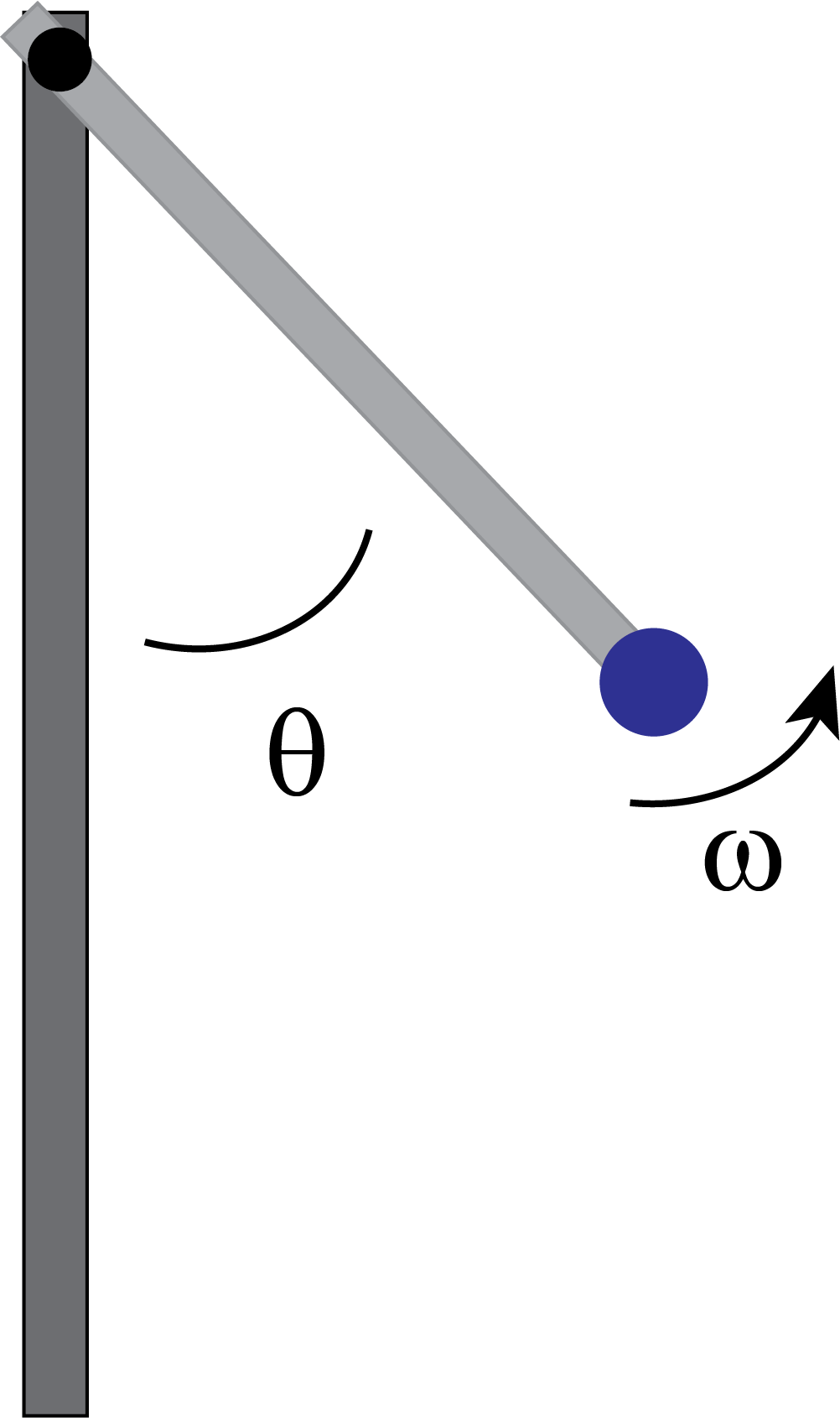
Of course, many biological, physical, and social systems require more than one variable to define a state. Even a simple pendulum represented by a ball of mass m attached to a massless, rigid rod with a pivot point so that the ball moves in a plane requires two variables to describe the state of the system, the angle \(\theta\) measured with respect to the vertical and the angular velocity \(\omega\). Figure 1.6 shows the geometry.
The more general dynamical system can be described by N state variables, \(y_0,\dddot ,y_{N- 1}\), and N rate equations, one for each state variable.
\[\begin{array}{l} \frac{dy_0}{dt} = f_1\left(t,y_0,\cdots, y_{N- 1},\mathbf p_0\right) \\ \vdots \\ \frac{dy_{N- 1}}{dt} = f_{N- 1}\left(t,y_0,\cdots, y_{N- 1},\mathbf p_{N- 1}\right) \\ \end{array} \tag{1.10}\]
Again, we assume that the functions \(f_0,\ldotp \ldotp \ldotp ,f_{N- 1}\) are known. If the state variables are known at a particular time, \(t=0\), for example, then the differential equations can be solved to give the state variables at subsequent times.
Numerical Solution of a Dynamical Systems Model
Solving a dynamical system model so that state variables can be predicted for some range of t values requires solving an ordinary differential equation, Equation 1.9, or a system of such equations, Equation 1.10. For some choices of the function f, or series of functions f0, …, fN-1, techniques from the theory of ordinary differential equations can be used to obtain explicit solutions for y or \(y_0,\ldots ,y_{N - 1}\). For example, consider the rate equation that leads to exponential growth.
\[\frac{dy}{dt} = ry\left(t\right) \label{eq:EquationExpGrowthModel} \tag{1.11}\]
Using elementary methods from calculus, this differential equation can be integrated to obtain
\[y\left(t\right) = y\left(0\right)e^{rt} \tag{1.12}\]
where y(0) is the value of y at \(t=0\).
We will often encounter dynamical systems models for which an explicit solution for the state variables cannot be obtained, at least not by the scientist or engineer who needs to use the solution. For such models, a numerical solution can be obtained through a numerical integration of the differential equation. We will not discuss here the mathematics behind developing such techniques but will present one method for using these techniques. The mathematics behind the numerical methods we will use is discussed by Iserles (Iserles, 2009). A powerful method for doing the numerical solution is to use the solveivp function from the scipy.integrate library (The SciPy Community, 2022). Figure 1.7 gives the basic template for using solveivp for a one-state variable model, as shown in Equation 1.9.
"""
Program Name: Exponential Growth Model: Numerical Solution
Author: C.D. Wentworth
version: 3.17.2020.1
Summary: Basic script for solving a dynamical system representing
         exponential growth. A numerical integration technique is
         used.

"""

import scipy.integrate as si
import numpy as np
import matplotlib.pylab as plt

def f(t,y,r):
#   y = a list that contains the system state
#   t = the time for which the right-hand-side of the system equations
#       is to be calculated.
#   r = a parameter needed for the model
#
    import numpy as np

#   Unpack the state of the system
    y0 = y[0] # cell density

#   Calculate the rates of change (the derivatives)
    dy0dt = r*y0

    return [dy0dt]
# Main Program

# Define the initial conditions
yi = [0.021]

# Define the time grid
t = np.linspace(0,300,200)

# Define the model parameters
r = 0.014
p = (r,)

# Solve the DE
sol = si.solve_ivp(f,(0,300),yi,t_eval=t,args=p)
ys = sol.y[0]

# Plot the theory
plt.plot(t,ys,color='g')
plt.xlabel('t [min]')
plt.ylabel('OD')
plt.savefig('ExponentialGrowth.png',dpi=300)
plt.show()As the code shows, you must define a Python function that calculates the right hand side of the rate equation defined in Equation 1.9 in terms of t and the current value of the state variable y, symbolized by the parameter \(y\) in \(f(t,y,r)\). You must also define the initial value \(y(0)\), called yi in the program, and a list of t values for which you need the value of the state variable \(y\left(t\right)\), which is done in line 37. The function solveivp returns a list of objects, contained in sol, that defines the solution. The solution corresponding to the times in the array t are contained in the array sol.y[0]. To use the solution values in a plot we extract the actual solution values from sol and name the array ys, in line 45. If the dynamical systems model had more than one state variable then we could extract the solution values for each state variable as shown below.
ys0 = sol.y[0]
ys1 = sol.y[1]
.
.
.
We will see an example of doing this in the next chapter. If the model has more than one parameter, they must all be placed in the tuple p in line 41 but listed separately in the function definition. The next section will show an example of such a model.
Computational Problem Solving: Mathematical Model for the Growth of Pseudomonas aeruginosa
To illustrate the numerical solution of a dynamical systems model we will return to the problem presented at the beginning of the chapter: the growth of Pseudomonas aeruginosa in a container with a fixed amount of liquid growth medium. When our goal is to develop a mathematical model of a system, we will use a modification of our four-step computational problem-solving strategy. Our strategy is
Analyze the problem
Formulate a model
Solve the model
Verify and interpret the model’s solution
Report on the model
Maintain the model
Analyze the Problem
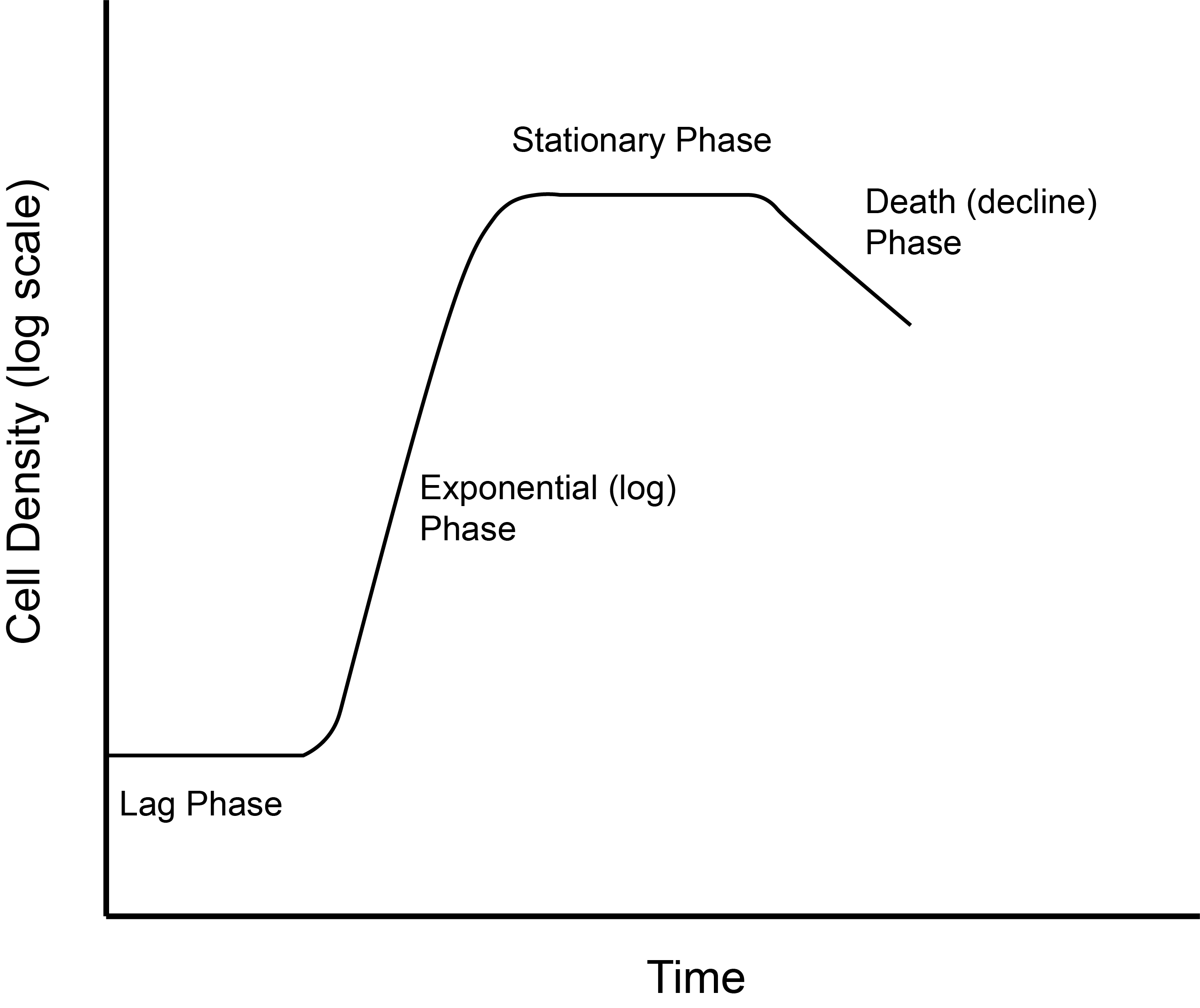
Our analysis begins with some library research on growth of microorganisms. We find that the typical stages of growth for bacteria in a container with fixed amount of growth medium are those shown in Figure 1.8. This is supposed to be a semi-log plot with the y-axis being the log axis. On such a plot, exponential growth appears as a straight line (Hardy, 2002).
For now, we will concentrate on modeling the exponential phase of cell growth. What factors in the system might affect the growth? In general, we might expect the temperature, pH, and other environmental factors will influence growth. We will assume those environmental factors are held constant. We are being very restrictive in how we describe the system. This is typical in starting a modeling project. We start with simple models and work our way up in complexity. In our case, there is one state variable:
\[y\left(t\right) \equiv \text{number of cells per ml}\]
What will determine the rate of change of \(y\left(t\right)\)? A reasonable hypothesis is that the rate of change of y will depend on the current number of cells, or cell density, that are present.
Formulate a model
We can express the hypothesis stated above with Equation 1.11, repeated below.
\[\frac{dy}{dt} = ry\left(t\right) \tag{1.13}\]
Solve the model
The model defined by Equation 1.13 can be solved with a little bit of calculus to give
\[y\left(t\right) = y\left(0\right)e^{rt} \tag{1.14}\]
This is the exponential growth model.
We will implement a numerical solution below since it is more common for the scientist or engineer to require such an approach.
Verify and interpret the model’s solution
We have data for the state variables with which to compare the predictions from the model. This is the ideal way of verifying the model. The data used to produce Figure 1.1 is in the file PA01SuspCell0p25PerCentGlucose-3-2017.txt. This data uses optical density of the liquid in the growth container to represent the cell density. Optical density is usually proportional to the actual cell density but establishing the exact relationship can be time-consuming.
The code in Figure 1.7 can be adapted to display both the theory and the data. Since the data file is composed of simple numerical columns we use the loadtxt function from Numpy to read in the data rather using Pandas. We can get the initial value of the state variable from the first row of data in the file. The value of the growth rate, r, is adjusted through trial and error to improve the fit between model and data. Figure 1.9 shows the adapted code. We will use statistical methods in Chapter 10 to find the best-fit model parameters. Figure 1.10 shows the comparison of the model and data.
"""
Program Name: PA01 Growth - Model and Data
Author: C.D. Wentworth
version: 8.16.2022.1
Summary: This program performs a numerical solution for the exponential
         growth dynamical systems model and compares the model results
         with actual growth data for PA01.
History:
    8.16.2022.1: base

"""

import scipy.integrate as si
import numpy as np
import matplotlib.pylab as plt

def f(t, y, r):
    #   y = a list that contains the system state
    #   t = the time for which the right-hand-side of the system equations
    #       is to be calculated.
    #   p = a tuple with parameters needed for the model
    #
    import numpy as np

    #   Unpack the state of the system
    y0 = y[0]  # cell density

    #   Calculate the rates of change (the derivatives)
    dy0dt = r * y0
    return [dy0dt]

# Main Program

# Read in data
cols = np.loadtxt('PA01_SuspCell_0p25PerCentGlucose_5-3-2017.txt',skiprows=6)
timeData = cols[:,0]
ODData = cols[:,1]

# Define the initial conditions
yi = [0.074]

# Define the time grid
t = np.linspace(0, 400, 200)

# Define the model parameters
r = 0.01175
p = (r,)

# Solve the DE
sol = si.solve_ivp(f, (0, 400), yi, t_eval=t, args=p)
ys = sol.y[0]

# Plot the theory and data
plt.plot(t, ys, color='g', label='Model')
plt.plot(timeData, ODData, linestyle='', marker='d',
         markersize=5.0, color='blue', label='Data')
plt.xlabel('t [min]')
plt.ylabel('OD')
plt.yscale('log')
plt.title('PA01 Growth: Comparison with Exponential Growth Model',
          fontsize= 12)
plt.legend()
plt.savefig('PA01_ExpGrowth_ModelAndData.png', dpi=300)
plt.show()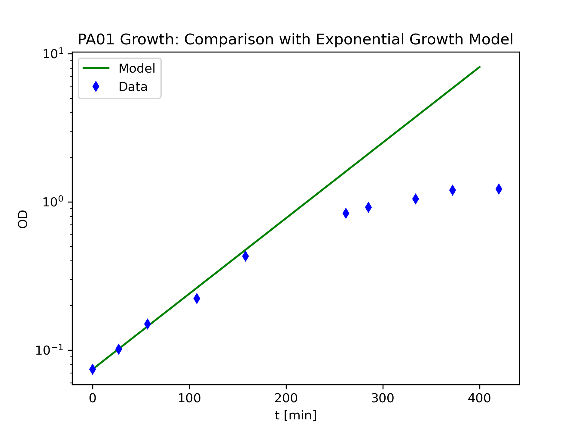
The exponential growth model shows a clear deficiency in describing the PA01 growth data for \(t>200[\text{min}]\). We can improve our model by including the effect of a finite amount of nutrients. At some point there will not be enough nutrients to allow cells to grow and divide. We must replace the rate equation Equation 1.13 with one that shows exponential growth for the rate equation for small values of y but eventually has the rate go to zero. One possible hypothesis is
\[\frac{dy\left(t\right)}{dt} = ry\left(1- \frac{y}{M}\right) \tag{1.15}\]
M is a new model parameter that represents the carrying capacity of the growth environment. When y approaches M, the rate of change for y will go to zero. The rate equation in Equation 1.15 is a historically famous one that defines the logistics model. Calculus techniques can be used to solve this differential equation exactly yielding Equation 1.16.
\[y\left(t\right) = \frac{My\left(0\right)e^{rt}}{M + y\left(0\right)(e^{rt}- 1)} \tag{1.16}\]
Instead of using the exact solution of Equation 1.15 we will implement a numerical solution so as to gain a little more experience in setting up the numerical solution framework.
"""
Program Name: PA01 Growth - Logistics Model and Data
Author: C.D. Wentworth
version: 8.16.2022.1
Summary: This program performs a numerical solution for the logistics
         growth dynamical systems model and compares the model results
         with actual growth data for PA01.
History:
    8.16.2022.1: base

"""

import scipy.integrate as si
import numpy as np
import matplotlib.pylab as plt

def f(t, y, r, M):
    #   y = a list that contains the system state
    #   t = the time for which the right-hand-side of the system equations
    #       is to be calculated.
    #   r = the specific growth rate
    #   M = the carrying capacity
    #
    import numpy as np

    #   Unpack the state of the system
    y0 = y[0]  # cell density

    #   Calculate the rates of change (the derivatives)
    dy0dt = r * y0 * (1.0 - y0/M)
    return [dy0dt]

# Main Program

# Read in data
cols = np.loadtxt('PA01_SuspCell_0p25PerCentGlucose_5-3-2017.txt', skiprows=6)
timeData = cols[:, 0]
ODData = cols[:, 1]

# Define the initial conditions
yi = [0.074]

# Define the time grid
t = np.linspace(0, 415, 200)

# Define the model parameters
r = 0.014
M = 1.25
p = (r, M)

# Solve the DE
sol = si.solve_ivp(f, (0, 415), yi, t_eval=t, args=p)
ys = sol.y[0]

# Plot the theory and data
plt.plot(t, ys, color='g', label='Model')
plt.plot(timeData, ODData, linestyle='', marker='d',
         markersize=5.0, color='blue', label='Data')
plt.xlabel('t [min]')
plt.ylabel('OD')
plt.yscale('log')
plt.title('PA01 Growth: Comparison with Logistics Growth Model',
          fontsize=12)
plt.legend()
plt.savefig('PA01_LogisticsGrowth_ModelAndData.png', dpi=300)
plt.show()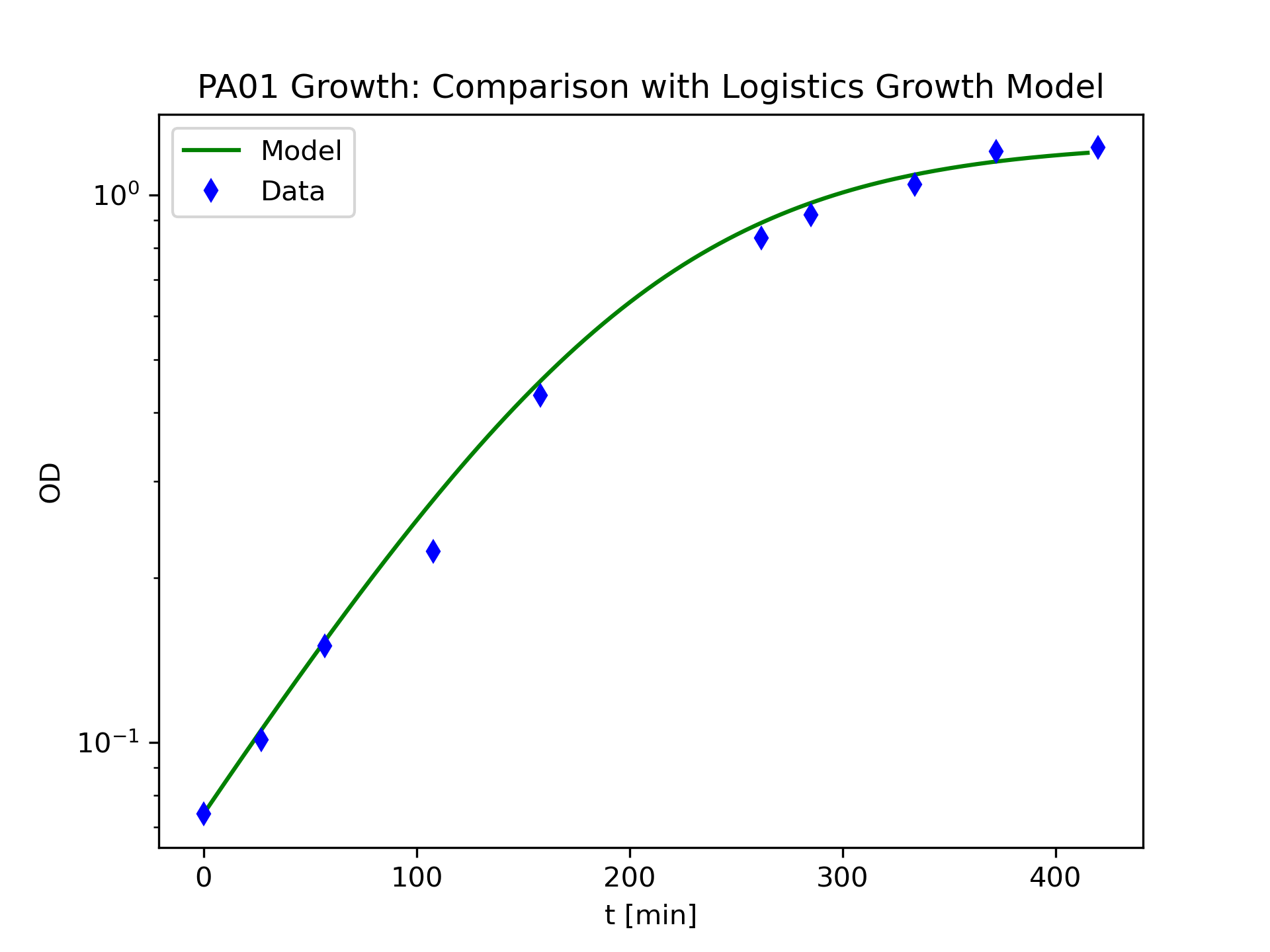
Report on the model
We used two different dynamical systems models to describe the PA01 bacteria growing in a glucose medium. The exponential growth model described by Equation 1.13 did not compare well with the available data over the time period in the data set, as can be seen in Figure 1.10. The logistics model given by Equation 1.15 described the available data well, as seen in Figure 1.12. The model parameter values that are appropriate for the PA01 strain of Pseudomonas aeruginosa grown in a 0.25% glucose minimal medium at 37 [C] are
\[\begin{array}{l} r = 0.014\left[{\min}^{- 1}\right] \\ M = 1.25\left[\text{OD units}\right] \\ \end{array}\]
Maintain the model
If we could obtain growth data over a longer period of time, then we would see the stationary phase give way to the death phase. We would then need to develop a more sophisticated model that could account for this phase. This could be the subject of a future research project.
Exercises
1. A dynamical system is one that changes with ____.
2. Select the statements that are true for a mathematical dynamical systems model.
- The state of the system is described by a set of time-dependent variables.
- The time rate of change of each state variable must be known.
- The current state of the system does not depend on the past state.
- It is a stochastic model.
3. T/F: The solve_ivp function can solve a first-order differential equation using numerical methods.
4. Calculate the integral of v(t) from t = 0 to t = 2 [s] where v(t) is shown in the figure below.
5. Write a short Python program that will calculate the derivative of the function
\[f\left(x\right) = \left(3x + 2x^3\right)\cos \left(x\right)\]
at \(x=2\). Use the cosine function in the Numpy module.
6. Write a short Python program that will calculate the integral from \(0 \leq x \leq 4\) of the following function
\[f\left(x\right) = \left(3x + 2x^3\right)\cos \left(x\right)\]
Program Modification Problems
1. Your goal is to use a numerical solution to an exponential growth model to simulate bacteria growth in an unconstrained environment (plenty of food) and find the growth rate parameter for Escherichia coli grown in CSHA media. Start with the code in Ch7ProgModProb1.py . Add a section that reads in the growth data in BacterialGrowthData.txt. Make sure you read in the column with the CSHA optical density measurement. Calculate the exponential growth model values for the optical density over the same time period as the data. Plot the data on the same graph. Change the value of the growth rate parameter and make the theory fit the data as best as you can.
Your plot should have the following features:
The theoretical (exponential growth model) values should be plotted with a solid green line.
The data points should be plotted using a filled circle as the marker. Make the color red and the size 8.
Add an appropriate title.
Save the graph as a png file.
2. Your goal is to use a numerical solution to a logistics growth model to simulate bacteria growth in a constrained environment (limitation in food) and find the growth rate parameter and carrying capacity for Vibrio natriegens grown in TSB media. Start with the code in Ch7ProgModProb2.py .
Change the import data section that reads in the growth data in V_natriegensGrowthData.txt. Make sure you read in the column with the TSB optical density measurement.
Change the function \(f\left(t,y,r\right)\) to implement the logistics model rate equation.
Change the initial condition.
Change the model parameter tuple p so that it contains both the growth rate r and the carrying capacity M.
Change the value of the growth rate parameter and carrying capacity and make the theory fit the data as best as you can.
Create a plot of both theory and data on the same graph. Your plot should have the following features:
The theoretical (logistics model) values should be plotted with a solid green line.
The data points should be plotted using a triangle as the marker. Make the color red and the size 8.
Save the graph as a png file.
Program Development Problems
1. Develop an argument that the numerical solution of a dynamical system model that we are using is valid. This will involve choosing a specific model for which we know the exact solution. The exponential growth model would be one choice. Next, create a program that solves the model numerically, add a function that calculates the exact solution, and then create a table that compares the numerical and the exact values for 10 values of the independent variable. Write a brief essay that summarizes your evidence that the numerical solution method is valid.
2. Solve the following first-order differential equation with the given initial condition by developing a Python program that can solve the equation numerically.
\[\frac{dy\left(t\right)}{dt} = \frac{\left(e^{rt}- 2y\left(t\right)\right)}{\left(1 + y^2\left(t\right)\right)}\text{,}y\left(0\right) = 0\]
Your program should make a plot of the solution for \(0 \leq t \leq 5\) and for r1 = 0.1 and r2 = 0.5 . The plot should have a solid blue continuous line for the model solution with r1 and a solid red line for the model solution with r2 . Add appropriate axis titles, a legend, and a chart title (y(t) versus t).
References
Diggle, S. P., & Whiteley, M. (2020). Microbe Profile: Pseudomonas aeruginosa: opportunistic pathogen and lab rat. Microbiology, 166(1), 30–33. https://doi.org/10.1099/mic.0.000860
Hardy, S. P. (2002). Chapter 2: Bacterial Growth. In Human Microbiology. Taylor & Francis.
Iserles, A. (2009). A first course in the numerical analysis of differential equations (2nd ed., Vol. 1–1 online resource (xviii, 459 pages) : illustrations). Cambridge University Press; WorldCat.org. http://www.books24x7.com/marc.asp?bookid=30922
The SciPy community. (2022a). . https://docs.scipy.org/doc/scipy/reference/generated/scipy.integrate.quad.html
The SciPy Community. (2022b). . https://docs.scipy.org/doc/scipy/reference/generated/scipy.integrate.solve_ivp.html
The SciPy community. (2026). . https://docs.scipy.org/doc/scipy/reference/generated/scipy.differentiate.derivative.html