Stochastic Models and Simulations
One way to categorize mathematical models of natural or engineered systems is to divide them into deterministic models or stochastic models. Deterministic models, such as the dynamical systems models we have considered previously, have no element of chance in their development. The exponential growth model for bacteria is an example. If we know how many bacteria are present at \(t=0\) and the growth rate r, then we can predict the number of bacteria precisely for \(t>0\) . Using Newton’s Second Law to predict the trajectory of a ball given the physical forces on it is another example. There are no probabilities or uncertainties about our theoretical predications based on these models. Stochastic models, involve an element of probability or randomness in their predictions. Here is a more formal definition.
Stochastic or probabilistic models use random variables to describe the system. Values for the random variables are based on theoretical or empirical probability distributions.
One example of a system that is best modeled using a stochastic model is the diffusive motion of individual atoms in a gas, liquid, or solid material for which there will be a probabilistic element. Other examples would include a dynamical systems model for which the model parameters are not known precisely but take on values with some probability.
If we want to simulate the behavior of a stochastic model, then we must perform numerical experiments that use random numbers selected according to an appropriate probability distribution. Such simulations are called Monte Carlo simulations, which we will explore in section 9.1. Random walks are a specific kind of Monte Carlo simulation that can be useful for modeling many systems. Another category of model we will explore in this chapter is cellular automata models. This class of models is not always stochastic in nature, but often is, so we include it here.
Motivating Problem: Comparing Betting Strategies at the Roulette Wheel
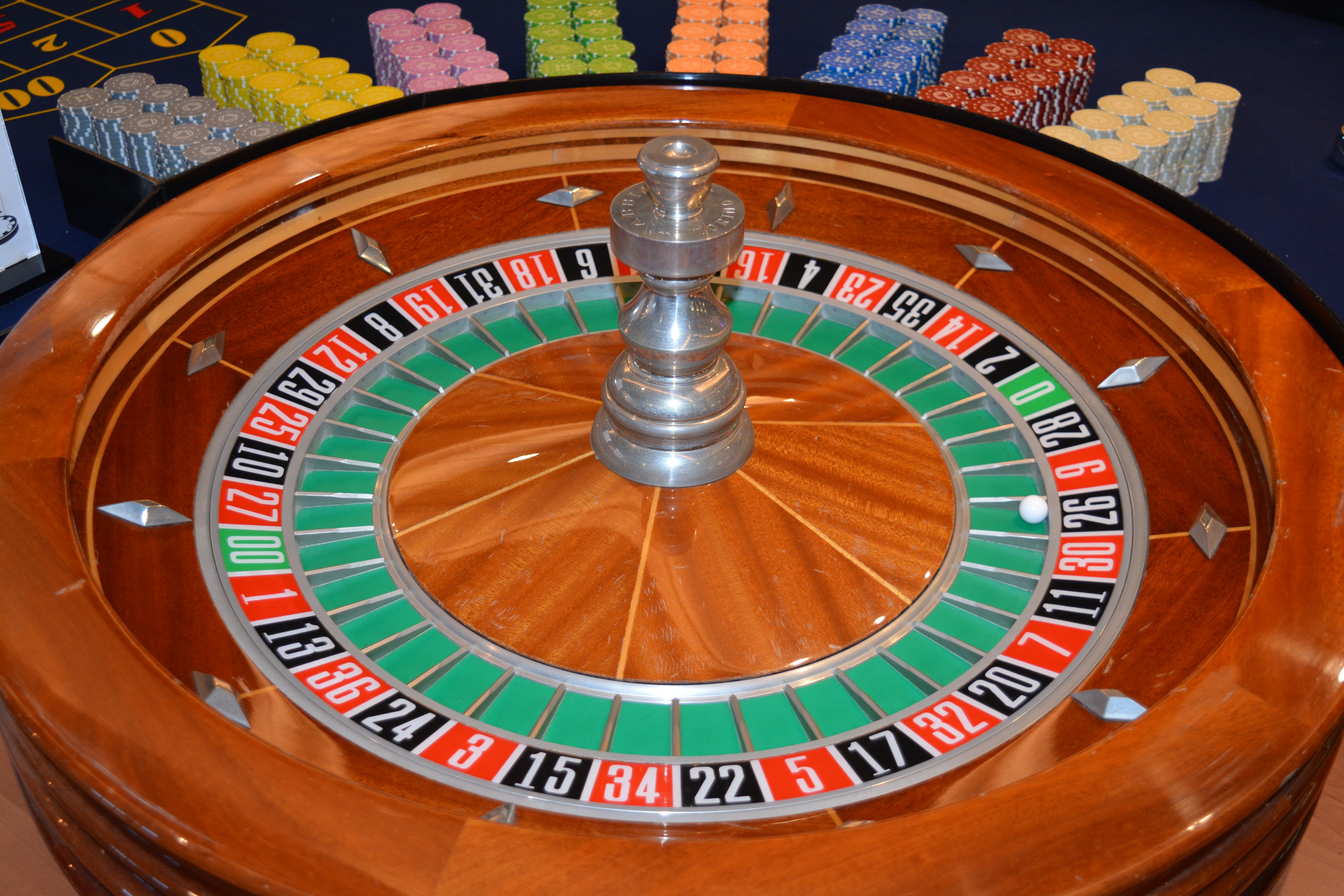
Let’s suppose you visit Las Vegas and want to play roulette. What kind of betting strategy should you employ so that you do not go broke? We can explore different strategies by using a computer simulation of a roulette wheel game. We want to develop a simulation for the American Roulette wheel shown in Figure 1. Roulette involves a long list of possible bets (Wikipedia Contributors, 2022), so we will use just a small subset of these and then explore some betting strategies such as the Martingale strategy or Anti-Martingale strategy.
Overview of Monte Carlo Methods
Definition
Stochastic models involve random variables. The behavior of the model will change depending on the specific values taken by the random variables in the model. Monte Carlo methods involve sampling the possible model behaviors from the set of all possible behaviors, which might by infinite, and then performing a statistical description of the behavior based on the set of samples. More succinctly, a Monte Carlo simulation involves repeated random sampling to explore the behavior of a system.
Generating Pseudorandom Numbers
To perform Monte Carlo simulations requires that computer programs have access to random numbers. The standard solution to this need is to actually use pseudorandom numbers, which are deterministically created lists of numbers that will pass a variety of statistical tests for lists of actual random numbers.
The pseudorandom number generators used by early computer programming languages used an algorithm known as a linear congruential generator. This algorithm is based on the following equation (Press et al., 1986).
\[I_j = \left(aI_{j- 1} + c\right)\mathrm{mod}m\]
The constants a, c, and m are chosen to yield acceptable statistical properties for the sequence \(I_0,I_1,I_2,\ldots\)To get the sequence started, the user usually provides a seed number, I0.
There are recognized statistical problems with linear congruential generators if long sequences or subsets of sequences are required (Entacher, 1998). Modern numerical packages now use more sophisticated algorithms to produce pseudorandom number sequences including the Mersenne Twistor algorithm (Matsumoto & Nishimura, 1998) and the permuted congruential generator algorithm (O’Neill, 2014). To understand these more sophisticated algorithms requires the reader have more background in statistics and probability theory than this book assumes, so we will not discuss how they work.
The Python random module uses the Mersenne Twistor algorithm to generate pseudorandom numbers (Python Software Foundation, 2022). The numpy.random package uses the permuted congruential generator algorithm (NumPy Developers, 2022).
The following are the important functions from the random module that we use.
random.seed(a=None)Initializes the random number generator. Any int can be used. If none is provided, then the system time is used. Using the same seed will generate the same sequence of pseudorandom numbers.
random.randint(a, b)Returns a random integer N such that \(a \leq N \leq b\).
random.random()Returns the next random floating point number in the range [0.0, 1.0).
random.gauss(mu, sigma)Returns a random number selected from the normal distribution, also called the Gaussian distribution. mu is the mean, and sigma is the standard deviation.
The following code is generally used to set up the random module for use in a program.
import random as rn
# initialize the generator
rn.seed(524287)
It is a good practice to explicitly set the seed so that a program gives reproducible results. This can be very helpful during the debugging phase of code development.
Numpy has its own random submodule. In versions before 1.17, the use of the Numpy random functions proceeded in much the same way as with the Python random module.
Numpy random module functions before Numpy version 1.17:
numpy.random.seed(a=None)Initializes the random number generator. Any int can be used for the value of a. If none is provided, then the system time is used. Using the same seed will generate the same sequence of pseudorandom numbers.
numpy.random.randint(a, b, size=None)Returns a random integer N such that \(a \leq N \leq b\). The size keyword argument can be provided a tuple that specifies the shape of a numpy array of random integers that will be returned.
numpy.random.random(size=None)Returns the next random floating point number in the range [0.0, 1.0). The size keyword argument can be provided a tuple that specifies the shape of a numpy array of random floats that will be returned.
numpy.random.normal(loc=0.0, scale=1.0, size=None)Returns a random number selected from the normal distribution, also called the Gaussian distribution. loc is the mean, and scale is the standard deviation. The size keyword argument can be provided a tuple that specifies the shape of a numpy array of random floats selected from the normal distribution that will be returned.
Starting with Numpy version 1.17, while the functions listed above can still be used, the best use recommendation has changed. The goal of the new version usage is to avoid problems with the seed being unintentionally reset by complex codes. The new approach allows separate copies (instances, to use Object Oriented Programming language) of the random number generator to be created that are independent of random number generators used in other modules. The following code shows how to create a copy of the random number generator.
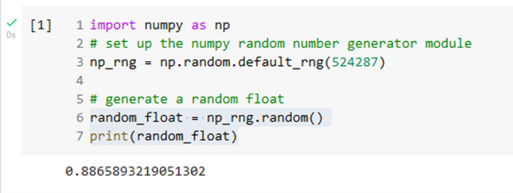
rng = numpy.random.default_rng(seed=None)The variable name rng will now refer to a separate copy of the numpy random module with scope restricted to the program unit in which it was defined. You can use any valid Python variable name instead of rng. If a seed number is not provided, then one generated from the computer operating system will be used.
Here is an example of code in a Jupyter notebook that uses the new Numpy random number generator approach.
Random Walks
Definition
A random walk is a process in which an object moves away from a starting position at random. Lattice random walks are a simple case of random walks where the object is assumed to move on a regular grid of sites. It is a series of steps taken in random directions. The steps can be considered to be taken in any kind of space that is of interest. In the simplest case, the walk starts at zero and then at each step a +1 or -1 is added to the current position to yield an updated position. The walk would be the list of integers giving the position at each time.
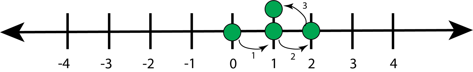
More generally, a random walk on a lattice envisions the walk occurring on a regular grid such as the one-dimensional grid shown in Figure 2. In a lattice random walk, each direction for taking a step is assigned a probability and at each time step the walker chooses a direction according to the assigned probability. Figure 2 shows one possible series of steps.
A Monte Carlo simulation of a random walk will execute many separate walks and then perform statistical analyses of whatever property that is of interest.
One-dimensional Random Walk
Let’s consider a simple situation that would not be described well by a deterministic model. Consider a bar with its entrance in a narrow alley. If someone exits the bar, then they can only move right, left, or stay in place. Now, imagine a man has been consuming alcoholic beverages in the bar for a couple of hours. Needless to say, he is rather intoxicated, so he decides to walk home (at least he knows not to drink and drive!). He leaves the bar, which means stepping into the alley where he can only move left or right. Given his level of intoxication, the man cannot think clearly or even walk in a straight line. He steps erratically left or right with no discernable pattern to his choice. His walk in the alley is random.
We will not be able to model this man’s walking behavior using a deterministic model, but we can still simulate the man’s motion using a stochastic model and look for possible patterns in his behavior. Models that simulate the behavior of a system based on an element of randomness are called Monte Carlo simulations. We will create a Monte Carlo simulation of the drunk man’s walking behavior called, appropriately enough, the random walk simulation. This type of model can be applied much more generally than simply describing the behavior of an intoxicated man, but this scenario is an easy one to visualize as we develop our understanding of stochastic simulations.
Recall our general problem-solving strategy:
Analysis: Analyze the problem
Design: Describe the data and develop algorithms
Implementation: Represent data using programming language data structures and implement the algorithms with specific programming language code
Testing: Test and debug the code using test data
Let’s analyze our problem: simulating the random walk of our intoxicated man. We note that the man can only move along the axis, so it is an inherently one-dimensional problem. The man will choose to take a step leftwards or rightwards with equal probability.
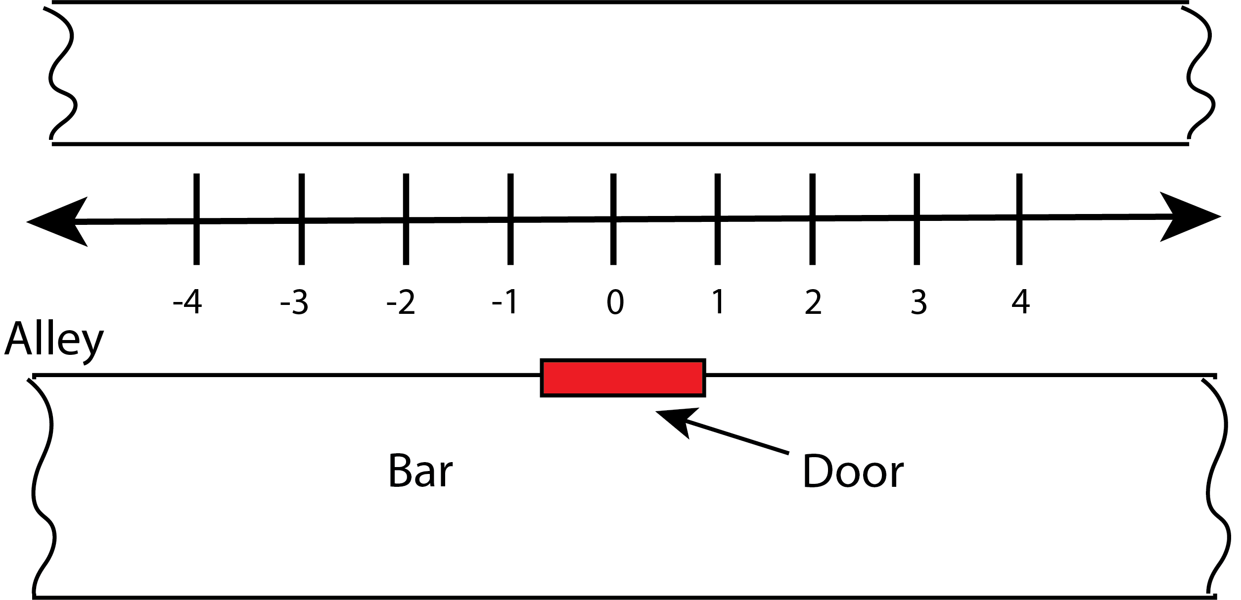
Now we will move on to designing our model. We will assume the man moves on the x-axis, as shown in Figure 3. His position at a particular time t is given by his x-coordinate, x(t). We will make the following simplifying assumptions:
The man attempts a step at equal time intervals.
The man chooses to step left or right with equal probability, like a coin toss.
All steps have length of 1 spatial unit.
Data structures:
N – total number of steps to simulate
i – the particular step currently being considered
xi – the position at step i
x_list – a list containing the position at each step
Here’s an initial pseudocode solution to the simulation:
PROGRAM randomWalk1d
    Initialize the drunk's position at the origin: xi = 0
    Set up a list to contain the drunk’s position at each step:
    defines x_list
    # set up a loop to execute N steps
    FOR i in the list (0,1,2,...N) DO
        Generate a random step
        Update xi
        Add xi to x_list
    ENDFOR
    Create a graph of position as a function of time
ENDPROGRAM
Let us take a more detailed look at the program step
Generate a random step
We will implement this step as a function named step(xi) that takes the current position xi and produces the next position, which is returned.
Here is a pseudocode version of the step(xi) function.
FUNCTION step
    INPUT: xi
    Choose a direction (left or right) at random
    IF left THEN
      xi = xi - 1
    ELSE
      xi = xi + 1
    ENDIF
    OUTPUT: xi
ENDFUNCTION
We will move on to the Implementation portion of our problem-solving strategy. Let us turn our attention to how we can generate random numbers in Python. The reality is that we cannot generate truly random numbers, but we can generate pseudorandom numbers that can pass tests for randomness as long as we do not try to generate too many of them.
We will use the Python random module to generate our pseudorandom numbers. We start our use of these functions with an import command:
import random as rn
One of the first steps in the main part of our program will be to set up the random number generator by providing a seed. We do this so that we can generate the same sequence of random numbers to aid in debugging the program.
So, how do we choose the left or right direction at random? We can use the random() function to generate a number between 0 and 1. If the number is less than 0.5 then we choose left for the direction. If the number is greater than or equal to 0.5 then we choose right for the direction. Here’s Python code for the step(xi) function:
def step(xi):
    r = rn.random()
    if r < 0.5:
        xi = xi -1
    else:
        xi = xi+1
    return xi
This code assumes the random module was imported and renamed rn by the main program.
A computer simulation of a random walk must assume a finite lattice size since the available memory for the simulation is finite. This fact means that we must decide how to handle the walker hitting a boundary. In the code being developed here, the step function must deal with the case of xi being on the boundary. There are two approaches to handling this situation. One is to assume reflective boundary conditions, which means that if the walker hits the boundary he just stays there. The other method is to use cyclic boundary conditions, which means that if the walker hits the boundary he actually goes to the other side, as if the x-axis wraps around on itself.
Let’s implement the reflective boundary conditions. We need to define two more variables:
lx – the lowest x value
ux – the highest x value
Here is the revised step function:
def step(xi,lx,ux):
r = rn.random()
if r < 0.5:
if xi >lx:
xi = xi - 1
else:
if xi < ux:
xi = xi + 1
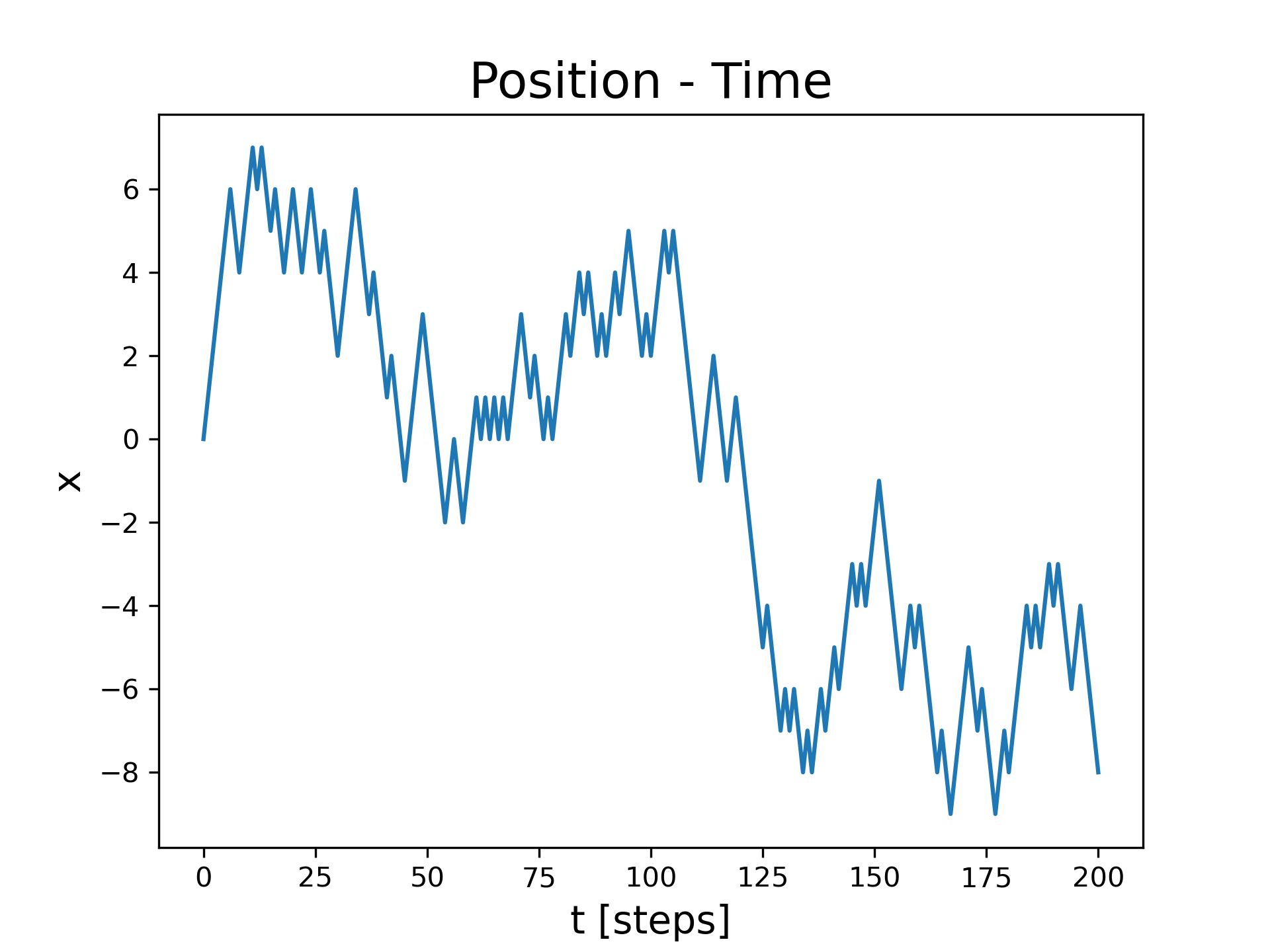
return xiA complete code for performing this one-dimensional simulation is shown in Figure 4. The code is in the chapter file randomWalk1d.py. This code produces a plot of the position as a function of time (step number) shown in Figure 5. The mean and standard deviation of the position is also calculated in lines 41-43.
"""
Program: 1-d Random Walk
Author: C.D. Wentworth
Version: 9.23.2022.1
Summary:
        This program performs a 1-dimensional random
        walk simulation.
History:
    9.23.2022.1: base
"""
import matplotlib.pyplot as plt
import numpy as np
import random as rn

def step(xi,lx,ux):
    import random as rn
    r = rn.random()
    if r < 0.5:
        if xi > lx:
            xi = xi -1
    else:
        if xi < ux:
            xi = xi+1
    return xi
# Main Program

# set up the grid
lx = -100
ux = 100

# set up random generator
rn.seed(524287)
N = 200

# execute random walk
xi = 0
xlist = [xi]
for i in range(N):
    xi=step(xi,lx,ux)
    xlist.append(xi)
xnp = np.array(xlist)
xmean = xnp.mean()
xsd = np.sqrt(xnp.var()/float(N-1))

# create plot of x - t
plt.plot(xlist)
plt.xlabel('t [steps]', fontsize=14)
plt.ylabel('x', fontsize=14)
plt.title('Position - Time', fontsize=18)
plt.savefig('randomwalk1d.png', dpi=300)
plt.show()

# print position
print('mean x = ',xmean,' sd = ',xsd)
print('final position x = ', xlist[-1])
|

|
Another important random walk property to study is how the distance of the walker to the origin varies with time. For a one-dimensional random walk that starts at the origin, the distance to the origin is given by
\[D = \left|x\right|\]
Figure 6 shows the distance as a function of time for a one-dimensional random walk on a grid defined by \(- 1000 < x < 1000\).
While the distance appears to increase with time, there is a significant amount of noise in this property. This is a typical result for any measured property in a stochastic simulation just as it is for a measurement taken in a real world experiment. To obtain a better picture of the distance as a function of time we should repeat the experiment, that is the simulation, many times and calculate the mean distance as a function of time where the mean is calculated from our sample of many simulations.
The key data structure for calculating the mean distance as a function of time is a numpy array that contains the distance to the origin at each time for each of the separate simulations. Table 1 shows the structure of this array.
| D11 | D12 | D13 | … | D1S |
|---|---|---|---|---|
| D21 | D22 | D23 | … | D2S |
| D31 | D32 | D33 | … | D3S |
|
. . . |
. . . |
. . . |
. . . |
. . . |
| DN1 | DN2 | DN3 | … | DNS |
\[D_{tn} = \text{distance at time }t\text{ for simulation }n\]
The mean distance at any particular time is calculated by averaging over all the columns of the row corresponding to the time of interest. Figure 7 shows the revised code that performs repetitions of the simulation and then calculates the mean distance as a function of time. Figure 8 shows a plot of the mean distance as a function of time (number of steps). Most of the random variation shown in Figure 6 has disappeared.
"""
Program: 1-d Random Walk - Multi Sims Version
Author: C.D. Wentworth
Version: 9.24.2022.1
Summary:
        This program performs a 1-dimensional random
        walk simulation. It performs multiple simulations
        and calculates the mean distance to the origin at each time.
History:
    9.24.2022.1: base
"""
import matplotlib.pyplot as plt
import numpy as np
import random as rn


def step(xi, lx, ux):
    import random as rn
    r = rn.random()
    if r < 0.5:
        if xi > lx:
            xi = xi - 1
    else:
        if xi < ux:
            xi = xi + 1
    return xi


# Main Program

# set up the grid
lx = -1000
ux = 1000

# set up random generator
rn.seed(524287)

# set up the simulations
N = 500  # number of steps in a simulation
S = 5000  # number of simulations
D_array = np.empty((N + 1, S), dtype='float')  # distance storage

for s in range(S):
    # execute random walk
    x0 = 0
    x = x0
    D_array[0, s] = 0.0
    for t in range(1, N + 1):
        x = step(x, lx, ux)
        D = np.abs((x - x0))
        D_array[t, s] = D

# calculate the mean distance at each time step and plot D-t
DMean = np.mean(D_array, axis=1)
plt.plot(DMean, linestyle='-')
plt.xlabel('t [steps]', fontsize=14)
plt.ylabel('D', fontsize=14)
titleString = 'D-t Mean of ' + str(S) + ' Simulations'
plt.title(titleString, fontsize=18)
plt.savefig('randomWalk1d_D-t_mean.png', dpi=300)
plt.show()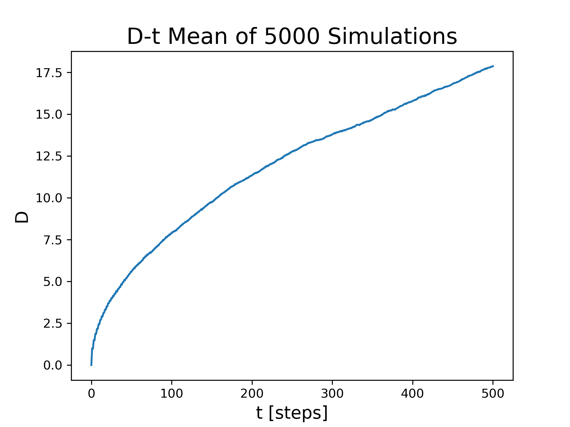
Two-dimensional Random Walk
Let’s give our intoxicated walker more room to roam around. We will place him in a large parking lot so that he can move about on a plane, a two-dimensional surface. We want to simulate his trajectory on the parking lot. Our model will be based on some simplifying assumptions, similar to the one-dimensional walk.
The man attempts a step at equal time intervals.
The man chooses to step north, south, east, or west with equal probability.
All steps have length of 1 spatial unit.
With these assumptions, our walker will roam about on a grid like chess pieces on a game board. The basic algorithm for performing the simulation will be the same as for the one-dimensional case. The major difference will be in the step function. It must now choose one of the four directions at random instead of either right or left. Here is a pseudocode version of the step function.
FUNCTION step
    INPUT: xi,yi
    Pick a random number r, from (1,2,3,4)
    IF r is 1 THEN
        Step east by incrementing xi
    ELIF r is 2 THEN
        Step west by decreasing xi
    ELIF r is 3 THEN
        Step north by increasing yi
    ELIF r is 4 THEN
        Step south by decreasing yi
    ENDIF
    OUTPUT: xi,yi
ENDFUNCTION
We must implement boundary conditions since the simulated grid will be finite. This will require minimum and maximum values for both the x and y coordinates. These values will be defined using the variables lx,ux,ly,uy. Figure 9 gives the Python code for the two-dimensional step function with reflective boundaries. Figure 10 shows an example of the overall trajectory of this random walk.
"""
Title: Random Walk in 2D: base
Author: C.D. Wentworth
version: 3-21-2019.1
Summary: This program performs a random walk on a
         two-dimensional lattice. It uses reflective
         boundary conditions.
version history:
        3-21-2019.1: base

"""
import matplotlib.pylab as plt
import numpy as np
import random as rn
import turtle as trt


def step(xi, yi, lx, ux, ly, uy):
    import random as rn
    r = rn.randint(1, 4)
    if r == 1:
        # go east
        if xi < ux:
            xi = xi + 1
    elif r == 2:
        # go west
        if xi > lx:
            xi = xi - 1
    elif r == 3:
        # go north
        if yi < uy:
            yi = yi + 1
    else:
        # go south
        if yi > ly:
            yi = yi - 1
    return xi, yi


# --Main Program
# set up random generator
rn.seed(42)

# define the grid
lx = -40
ux = 40
ly = -40
uy = 40

# set up the simulation
N = 1000
xi = 0
yi = 0
position_array = np.zeros((N + 1, 2))

# execute random walk
for i in range(1, N + 1):
    xi, yi = step(xi, yi, lx, ux, ly, uy)
    position_array[i, 0] = xi
    position_array[i, 1] = yi

x_array = position_array[:, 0]
y_array = position_array[:, 1]

# create plot
x0 = x_array[0]  # initial x
y0 = y_array[0]  # initial y
xf = x_array[-1]  # final x
yf = y_array[-1]  # final y
plt.plot(x_array, y_array)
plt.plot(x0, y0, linestyle='', marker='o', markersize=8,
         markeredgecolor='green', markerfacecolor='green')
plt.plot(xf, yf, linestyle='', marker='o', markersize=8,
         markeredgecolor='red', markerfacecolor='red')
plt.xlim(-20, 20)
plt.ylim(-20, 20)
plt.savefig('randomWalk2d.png', dpi=300)
plt.show()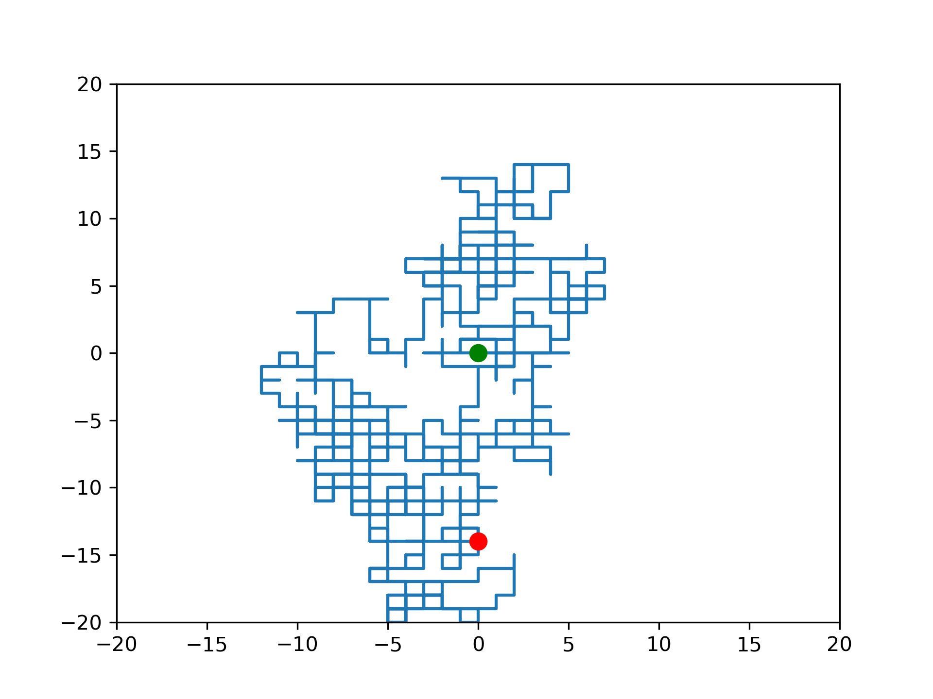
Cellular Automaton Model
Cellular automata can be considered as a particular abstract framework for describing the real world, that is, a modelling framework, or as a kind of mathematical object that can be used to build models or investigate computational problems (Berto & Tagliabue, 2022). We will start with a formal, mathematical definition of a cellular automaton. A cellular automaton model is defined as
a discrete lattice of sites or cells in d dimensions, L
operating using discrete time steps
a discrete set of possible cell values, S
a defined neighborhood, N of each cell in L
a transition rule, \(\Phi\), that specifies how the state of a cell will be updated depending on its current value and the values of sites in the neighborhood.
We will consider the cellular automaton to be the collection \(〈L,S,N,\Phi 〉\). A specific example will be defined in the next section, which should make this definition less abstract. Cellular automata have been used to model
computational machines
growth of biological systems such as biofilms
evolution of life
phase transitions in magnetic materials
urban development
Cellular automata are often used to show how complex patterns can be the result of simple rules governing the behavior of the system being considered.
Deterministic Cellular Automata
We will define a simple one-dimensional cellular automaton. The lattice L is an infinite, one-dimensional set of cells, as shown in Figure 11.

The possible cell values will be \(S = \left\{0,1\right\}\). We will visualize a cell with state 0 as white and state 1 as black. The neighborhood, N, of a cell will be defined as the nearest neighbors of the cell: the cell to the left and the cell to the right. A particular combination of neighbors and center will be symbolized by LCR.
The transition rule will be a new assignment of the C state based on the current value of the LCR combination. There are eight possible LCR combinations for this class of cellular automata, shown in Table 9.2. There are two possible new values for the C cell given a specific LCR combination. Therefore, there are 28 possible transition rules for this class of cellular automata.
We will enumerate each possibility by an integer from 1 to 256. The transition rule will be given by the binary representation of rule number given by the base 10 integer. For example, Rule 150 has the binary representation 10010110. Each of the eight digits in this representation gives the transition rule a specific LCR combination. Table 2 illustrates how this assignment can be made.
| L | C | R | new C |
|---|---|---|---|
| 1 | 1 | 1 | 1 |
| 1 | 1 | 0 | 0 |
| 1 | 0 | 1 | 0 |
| 1 | 0 | 0 | 1 |
| 0 | 1 | 1 | 0 |
| 0 | 1 | 0 | 1 |
| 0 | 0 | 1 | 1 |
| 0 | 0 | 0 | 0 |
Now we must construct a computer simulation of this simple cellular automaton model. We will base the code on one developed by Cyrille Rossant (Rossant, 2018).
| Variable | Type | Description |
|---|---|---|
| size | int | The number of cells in the lattice. |
| steps | int | The number of time steps to simulate. |
| rule | int | The state transition rule given as a decimal number. |
| rule_b | ndarray | The state transition rule given as a binary number represented in a numpy array. |
| x | ndarray | A 2d numpy array where each row gives the state of the cellular automaton at a specific time. The array contains the entire simulated evolution of the automaton. |
| LCR_array | ndarray | Each column of the array gives the Left, Center, and Right state values for a particular cell in the automaton. Used in step function. |
| xs | ndarray | A 1-dim array that gives the cell states for each cell in the automaton at one time. Used in the step function. |
Since the cellular automaton is being simulated by a computer, the lattice used to define the automaton must by finite. This means we must specify how the neighbors are defined for the cells all the way on the left and all the way on the right of the lattice. We will use periodic boundary conditions. This means that for the cell all the way on the left, the left neighbor will be the cell all the way on the right of the lattice. For the cell all the way on the right, the right neighbor will be the cell all the way on the left of the lattice. Figure 12 shows the code contained in the file CA_sim.py for simulating the simple one-dimensional cellular automaton. Figure 13 shows the output from the simulation for a Rule 150 cellular automaton with an initial state comprised of one active cell in the middle of the lattice.
"""
Program: 1-d Cellular Automaton Simulation
Author: Based on code from Rossant, C. (2018).
        IPython Interactive Computing and Visualization Cookbook—
        Second Edition. Packt Publishing.
        Revisions by C.D. Wentworth
Version: 9.29.2022.1
Summary:
        This program simulates a one-dimensional deterministic
        cellular automaton.
History:
    9.29.2022.1: base
"""
import numpy as np
import matplotlib.pyplot as plt

u = np.array([[4], [2], [1]])

def step(xs, rule_b):
    """
    Compute a single state of an elementary cellular
    automaton.
    """
    # Define the array that gives the LCR state values
    # for each cell.
    LCR_array = np.vstack((np.roll(xs, 1), xs,
                   np.roll(xs, -1))).astype(np.int8)
    # We get the LCR pattern numbers between 0 and 7
    # for each cell in the automaton.
    z = np.sum(LCR_array * u, axis=0).astype(np.int8)
    # We get the updated cell states given by the rule.
    return rule_b[7 - z]

def generate(rule, size=100, steps=100):
    """
    Simulate an elementary cellular automaton given
    its rule (number between 0 and 255).
    """
    # Compute the binary representation of the rule.
    rule_b = np.array(
        [int(_) for _ in np.binary_repr(rule, 8)],
        dtype=np.int8)
    x = np.zeros((steps, size), dtype=np.int8)
    # Define the initial state
    x[0, 50] = 1
    # Apply the step function iteratively.
    for i in range(steps - 1):
        x[i + 1, :] = step(x[i, :], rule_b)
    return x


# Main Program
rule = 150
size = 100
steps = 50
x = generate(rule, size, steps)
plt.matshow(x, cmap=plt.cm.binary)
title_string = 'Rule ' + str(rule)
plt.title(title_string, fontsize=18)
fig_file = 'CA_rule' + str(rule) + '.png'
plt.savefig(fig_file, dpi=300)
plt.show()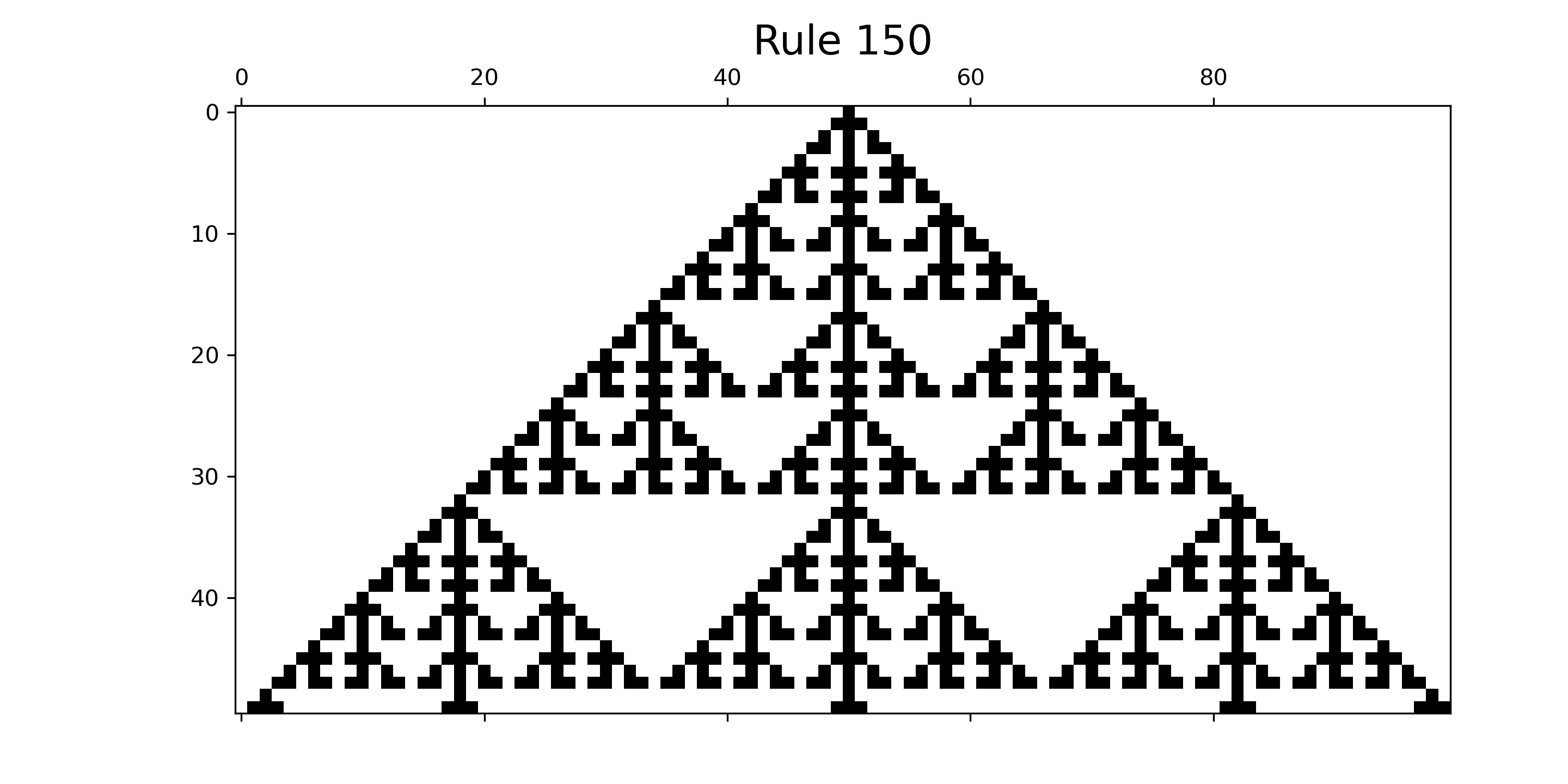
Probabilistic Cellular Automata
The cellular automata considered in the previous section are completely deterministic. Once the transition rule and initial state have been chosen the evolution of the lattice is determined. Repetition of the evolution will always yield the same result. We can introduce randomness in at least two ways:
create a random initial state or
establish a transition rule that updates the state of a cell using the neighborhood state and then a new cell state chosen according to a probability distribution.
Probabilistic cellular automata are usually defined using the second method of achieving randomness. We will not discuss coding of a probabilistic cellular automaton simulation here.
Computational Problem Solving: Comparing Betting Strategies at the Roulette Wheel
We began this chapter with the problem of comparing betting strategies when playing roulette. Let us return to that problem and develop a Monte Carlo simulation approach to solving the problem. We will consider playing American roulette and will restrict the betting types to a small subset of the possible ones.
Analysis
American roulette uses a wheel with 38 pockets that include both a 0 and a 00 pocket. The 0 and 00 pockets are green. The other pockets alternate between black and red. There are a large number of possible bets, so we will need to restrict the analysis to a small subset to facilitate the initial solution (Wikipedia Contributors, 2022). For this initial analysis, we will consider the following types of bets.
Straight/Single: bet on a single number; 35:1 payout
Red/Black: bet on either red or black; 1:1 payout
Green: bet on green; 17:1 payout
Each pocket of the wheel has numerical value, including 00, and a color. Table 4 gives the sequence of the slots going clockwise around the wheel. We will assume that when the wheel spins, the ball has an equal chance of falling into any one of the 38 pockets. For this initial attempt at simulating roulette, we will assume that each play involves a constant bet and a choice betting type. A game will be defined as a series of plays. For a game, the series of plays will end when the players balance goes below zero or if the balance goes above a specified balance value. Our gambler will continue playing until either they run out of money or until they achieve a specified level of profit.
| pocket index | value | color | pocket index | value | color | |
|---|---|---|---|---|---|---|
| 0 | 0 | green | 19 | 0 | green | |
| 1 | 28 | black | 20 | 27 | red | |
| 2 | 9 | red | 21 | 10 | black | |
| 3 | 26 | black | 22 | 25 | red | |
| 4 | 30 | red | 23 | 39 | black | |
| 5 | 11 | black | 24 | 12 | red | |
| 6 | 7 | red | 25 | 8 | black | |
| 7 | 20 | black | 26 | 19 | red | |
| 8 | 32 | red | 27 | 31 | black | |
| 9 | 17 | black | 28 | 18 | red | |
| 10 | 5 | red | 29 | 6 | black | |
| 11 | 22 | black | 30 | 21 | red | |
| 12 | 34 | red | 31 | 33 | black | |
| 13 | 15 | black | 32 | 16 | red | |
| 14 | 3 | red | 33 | 4 | black | |
| 15 | 24 | black | 34 | 23 | red | |
| 16 | 36 | red | 35 | 35 | black | |
| 17 | 13 | black | 36 | 14 | red | |
| 18 | 1 | red | 37 | 2 | black |
Design
Let us start the design of the algorithm by defining data structures that will be required. We will also create the roulette wheel data from Table 4 as columns in a tab-delimited text file. This file will be named wheel.txt. Table 5 gives a list of data structures that will be required for the roulette simulation.
| Variable | Type | Description |
|---|---|---|
| balance | int | This contains the current balance value of the gambler’s purse. |
| stop_balance | int | The balance value that will stop the game. Assumed to be larger than the starting value |
| bet_amount | int | |
| bet_type | str | Specifies whether the gambler is betting on a color (‘black’, ‘red’, green’) or a specific value (‘0’, ‘1’, …, ‘00’) |
| number_of_games | int | The number of repeated games to play, which will create the Monte Carlo simulation sample. |
| bet_types | dictionary | Associates the payout value with a bet type. |
| df | pandas data frame | Contains the wheel information read in from the wheel.txt file. |
| values | list | Contains all of the pocket values specified in the order found on the wheel going clockwise. |
| colors | list | Contains all of the pocket colors specified in the order found on the wheel going clockwise. |
| balance_series | list | Contains the balance value for each play in a game |
| spin_value | str | Contains the pocket value after a spin of the wheel. |
| spin_color | str | Contains the pocket color after a spin of the wheel. |
The following gives a pseudocode version of the main program for the simulation.
PROGRAM American_Roulette_Simulation-ConstantBetting
    Specify gambler’s data (balance, stop_balance, bet_amount,
                            bet_type, number_of_games)
    Initialize the random number generator
    Define the bet_types dictionary
    Define the wheel variables (values, colors)
    FOR g IN list_of_games DO
        Play a game
        Create a plot of the balance versus number of plays
    ENDFOR
ENDPROGRAM
The Play a game line will require another function, which we name game_constant_bet, and this function will require another function called make_a_play.
FUNCTION game_constant_bet
    INPUT: balance, stop_balance, bet_amount, bet_type, bet_types,
           values, colors
    balance_series = [balance]
    WHILE (balance > 0) and (balance < stop_balance) DO
        balance = make_a_play(balance, bet_amount, bet_type,
                              bet_types, values, colors)
        balance_series.append(balance)
    ENDWHILE
    OUTPUT: balance_series
ENDFUNCTION
The function game_constant_bet requires another function make_play.
FUNCTION make_a_play
    INPUT: balance, bet_amount, bet_type, bet_types, values, colors
    Perform a spin of the wheel (defines spin_value, spin_color)
    IF bet_type == 'black'
        IF spin_color == 'black'
            balance = balance + bet_amount*bet_types['black']
        ELSE
            balance = balance - bet_amount
        ENDIF
    ELIF bet_type == 'red'
        IF spin_color == 'red'
            balance = balance + bet_amount*bet_types['red']
        ELSE
            balance = balance - bet_amount
        ENDIF
    ELIF bet_type == 'green'
        IF spin_color == 'green'
            balance = balance + bet_amount*bet_types['green']
        ELSE
            balance = balance - bet_amount
        ENDIF
    ELSE
        IF spin_value == bet_type
            balance = balance + bet_amount*bet_types['value']
        ELSE
            balance = balance - bet_amount
        ENDIF
    ENDIF
    OUTPUT: balance
ENDFUNCTION
The function make_a_play requires a function which we call spin.
FUNCTION spin
    INPUT: values, colors
    Get a random integer between 0 and 37 (defines i)
    value = values(i)
    color = colors(i)
    OUTPUT: value, color
ENDFUNCTION
These pseudocode versions of the algorithm should allow an easy translation into Python code.
Implementation
Figure 14 gives the Python implementation of the American Roulette with Constant Bet simulation.
"""
Program: American Roulette with Constant Bet
Author: C.D. Wentworth
Version: 4.22.2025.1
Summary:
        This program performs a Monte Carlo simulation of the
        American roulette game using a constant bet strategy based
        either color choice or specific value choice.
History:
    9.01.2022.1: base
    4.22.2025.1: corrected make_a_play function
"""
import matplotlib.pyplot as plt
import numpy as np
import pandas as pd

def spin(values,colors):
#    i = rn.randint(0, 37)
    i = rng.integers(low=0 , high=37 )
    value = values[i]
    color = colors[i]
    return value, color

def make_a_play(balance, bet_amount, bet_type, bet_types,
                values, colors):
    spin_value, spin_color = spin(values, colors)
    if bet_type == 'black':
        if spin_color == 'black':
            balance = balance + bet_amount*bet_types['black']
        else:
            balance = balance - bet_amount
    elif bet_type == 'red':
        if spin_color == 'red':
            balance = balance + bet_amount*bet_types['red']
        else:
            balance = balance - bet_amount
    elif bet_type == 'green':
        if spin_color == 'green':
            balance = balance + bet_amount*bet_types['green']
        else:
            balance = balance - bet_amount
    else:
        if spin_value == bet_type:
            balance = balance + bet_amount*bet_types['value']
        else:
            balance = balance - bet_amount
    return balance

def game_constant_bet(balance, stop_balance, bet_amount, bet_type,
                      bet_types, values, colors):
    balance_series = [balance]
    while (balance > 0) and (balance < stop_balance):
        balance = make_a_play(balance, bet_amount, bet_type, bet_types,
                  values, colors)
        balance_series.append(balance)
    return balance_series


# Main Program
# Initialize gambler's data
balance = 1000
stop_balance = 1200
bet_amount = 10
bet_type = '15'
number_of_games = 100

# Set up the numpy random number generator
rng = np.random.default_rng(314159)

# Initialize the bet type payout
bet_types = {'black': 1, 'red': 1, 'green': 17, 'value': 35  }

# Read in the wheel data
df = pd.read_csv('wheel.txt', sep='\t', header=1,
       dtype={'index':int, 'value':'string', 'color':'string'})

# Convert pandas columns to tuples
values = tuple(df['value'].tolist())
colors = tuple(df['color'].tolist())

for g in range(number_of_games):
    balance_series = game_constant_bet(balance, stop_balance,
                                       bet_amount, bet_type,
                                       bet_types, values, colors)
    plt.plot(balance_series)
plt.xlabel('play')
plt.ylabel('balance')
title_string = 'Constant Bet Strategy: ' + bet_type
plt.title(title_string, fontsize=18)
plt.savefig('roulette_constantBet_value15_1200.png', dpi=300)
plt.show()This code is in the file roulette_constantBet.py.
Testing
A good strategy for testing the program is to create a series of small programs that test the individual functions. If the individual functions work as expected, then you will have some significant evidence that the overall program works as expected. Figure 15 shows a short code that will test the spin function. A write statement is inserted into the function to write out some test data to a file. Table 6 shows data generated by this code. The rows are compared with Table 4. After the test, lines 10-13 are deleted.
| pocket index | pocket value | pocket color | correct entry |
|---|---|---|---|
| 29 | 6 | black | yes |
| 4 | 30 | red | yes |
| 14 | 3 | red | yes |
| 32 | 16 | red | yes |
| 31 | 33 | black | yes |
| 28 | 18 | red | yes |
| 29 | 6 | black | yes |
| 2 | 9 | red | yes |
| 27 | 31 | black | yes |
| 3 | 26 | black | yes |
"""
Program: Test Spin Function
Author: C.D. Wentworth
Version: 9.1.2022.1
Summary:
        This program tests the spin function from the American
        Roulette Constant Bet simulation.
History:
    9.1.2022.1: base
"""
import matplotlib.pyplot as plt
import numpy as np
import pandas as pd
import random as rn

def spin(values,colors):
    i = rn.randint(0, 37)
    value = values[i]
    color = colors[i]
    # write test data
    write_string = str(i) + '\t' + value + '\t' + color + '\n'
    out_file.write(write_string)
    # end write test data
    return value, color


# Main Program
number_of_tests = 10

# Initialize random number generator
rn.seed(524287)

# Read in the wheel data
df = pd.read_csv('wheel.txt', sep='\t', header=1,
       dtype={'index':int, 'value':'string', 'color':'string'})

# Convert pandas columns to tuples
values = tuple(df['value'].tolist())
colors = tuple(df['color'].tolist())

out_file = open('testSpinFunctionData.txt', 'w')
for t in range(number_of_tests):
    value, color = spin(values, colors)
out_file.close()Similar short programs can be used to test the other functions.
To obtain some initial data for the constant bet strategy we will choose the following initial gambler’s data:
balance = 1000
stop_balance = 1200
bet_amount = 10
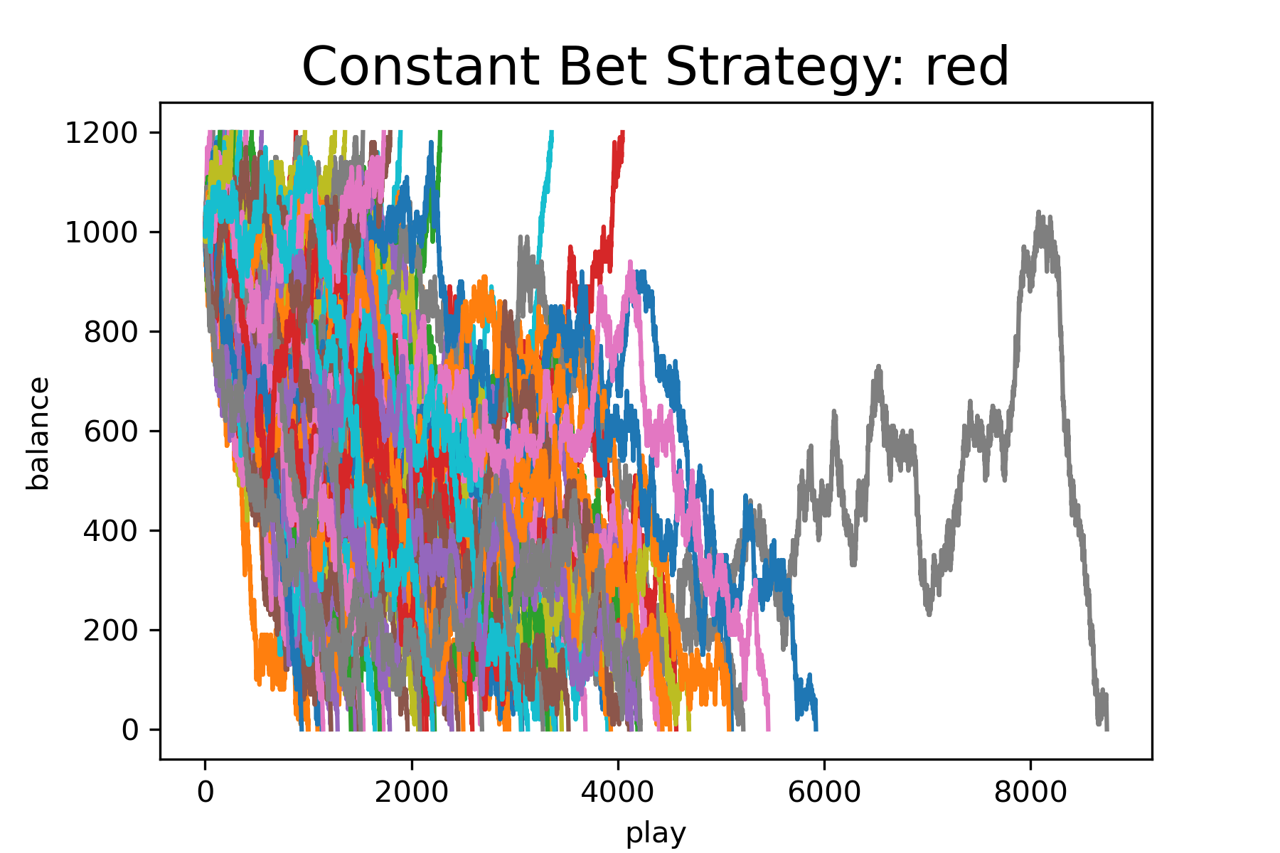
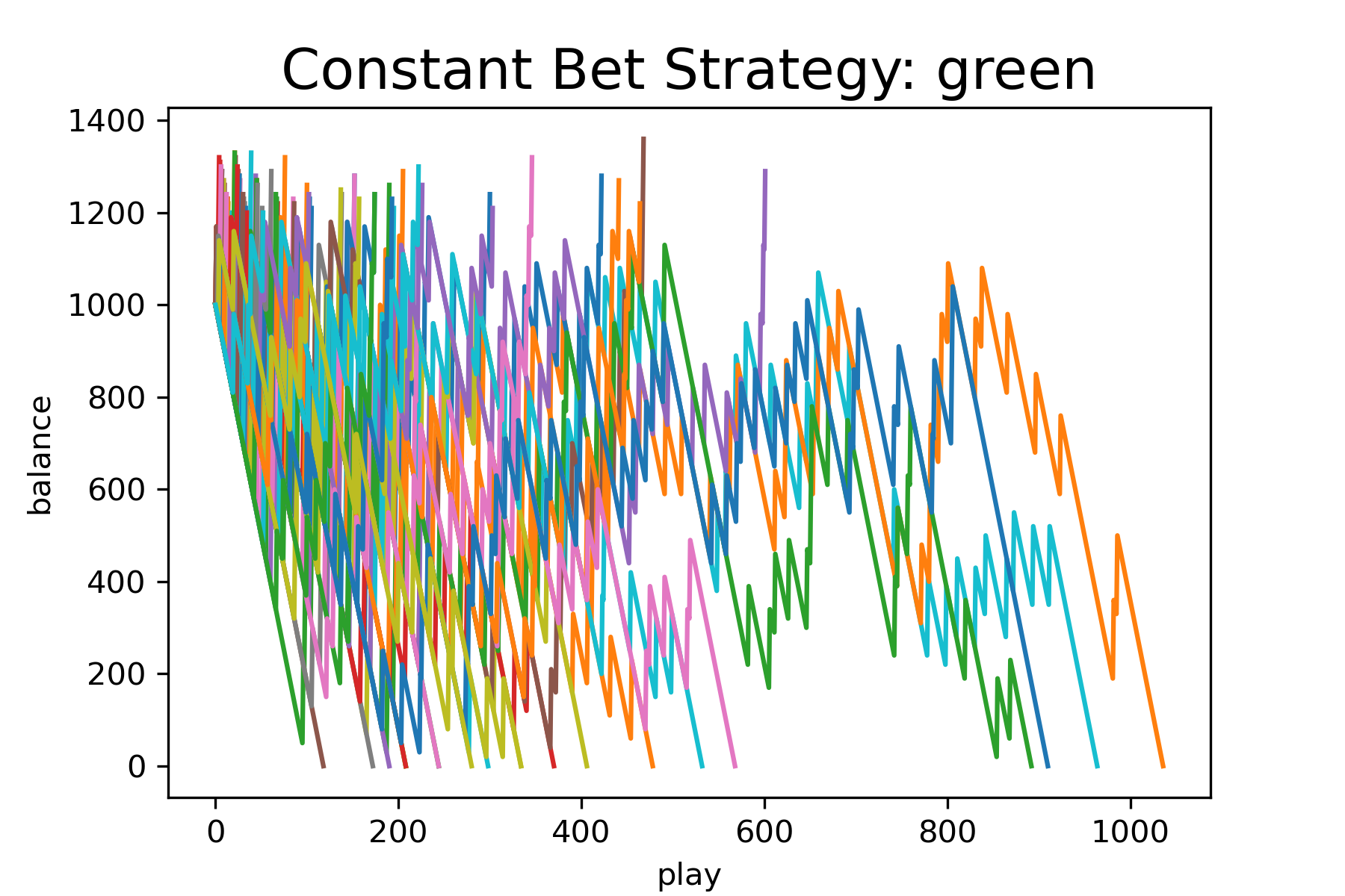
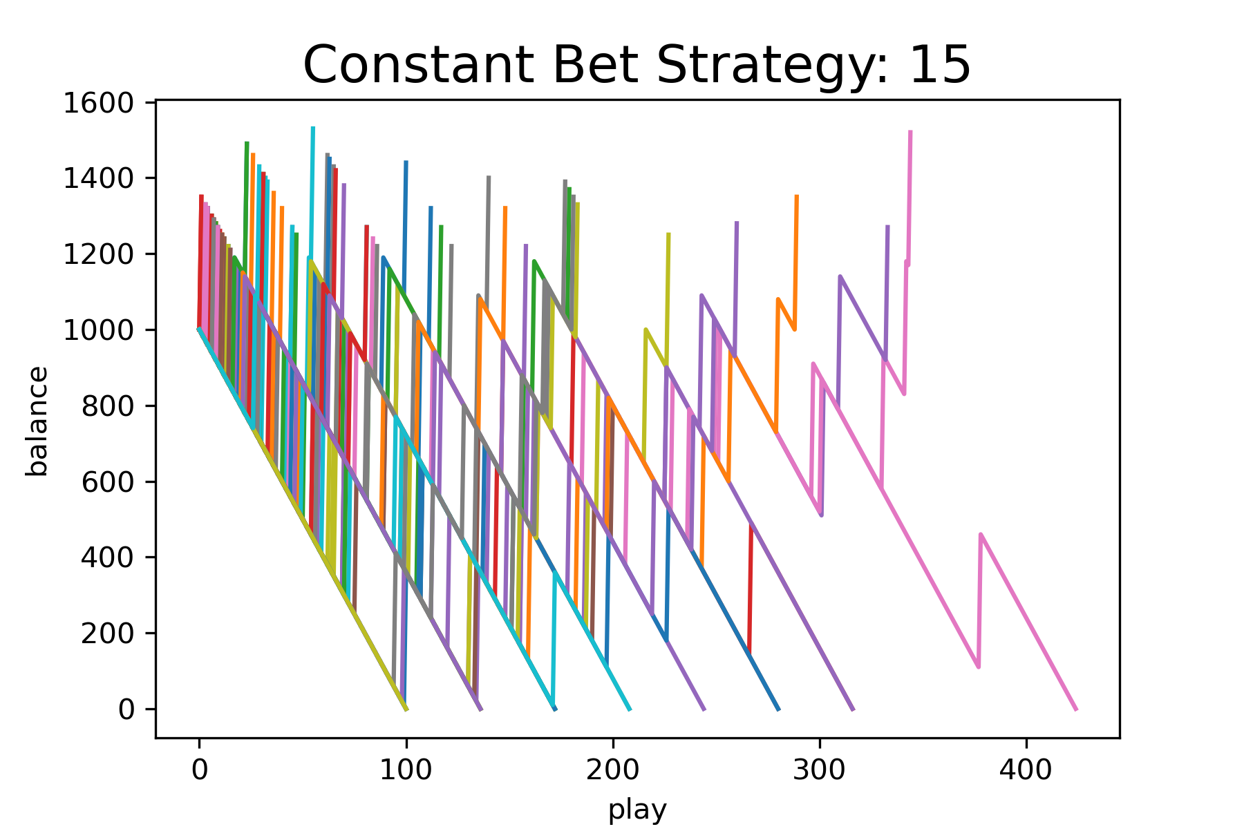
number_of_games = 100We will run the simulation for the following bet types: ‘red’, ‘green’, ‘15’, and compare the plots of balance as a function of play. Figure 16 – Figure 18 show the results of these simulations. Each simulation is for 100 games. Based on this data, a constant bet on red allows one to play longer before running out of money than the other bet types. A more thorough analysis that explores bet size effects and calculates the actual probability of reaching 1200 should be done before recommending the best version of the constant bet strategy.
Program Modification Problems
1. Starting with the two-dimension random walk code in Ch9ProgModProb1.py, write a program that calculates the distance to the origin of the walker as a function of step number (time). The program should produce a plot of D versus t. You can remove the plot of the actual walk.
2. Starting with the one-dimensional cellular automata simulation code in Ch9ProgModProb2.py, create a program that assigns an initial state of 1 to several randomly selected cells. Explore the differences in the patterns obtained between the revised program and the original one with initial state of 1 in the middle of the lattice.
3. Starting with the American Roulette with Constant Bet code in Ch9ProgModProb3.py, create a program to calculate the proportion of games that end with a profit for the bet on green and bet on a specific value bet types.
Program Development Problems
1. Create a program that simulates a two-dimensional random walk repeatedly and calculates the mean distance at each step over the sample of repeated simulations and produces a plot of mean distance as a function of step. The sample size should be large enough so that you get a smooth curve.
2. Create a program that will simulate the American roulette game using the Martingale strategy that involves doubling the bet value after losing a play. Explore the behavior of this strategy for the different betting types considered in the program American Roulette with Constant Bet contained in the file roulette_constantBet.py.
References
Berto, F., & Tagliabue, J. (2022). Cellular Automata. In E. N. Zalta (Ed.), The Stanford Encyclopedia of Philosophy (Spring 2022). Metaphysics Research Lab, Stanford University. https://plato.stanford.edu/archives/spr2022/entries/cellular-automata/
Derek Lynn. (2020). Roulette wheel in a casino for gambling entertainment [Photograph]. https://unsplash.com/photos/mD1V-eS1Wb4
Entacher, K. (1998). Bad subsequences of well-known linear congruential pseudorandom number generators. ACM Transactions on Modeling and Computer Simulation, 8(1), 61–70. https://doi.org/10.1145/272991.273009
Matsumoto, M., & Nishimura, T. (1998). Mersenne twister: A 623-dimensionally equidistributed uniform pseudo-random number generator. ACM Transactions on Modeling and Computer Simulation, 8(1), 3–30. https://doi.org/10.1145/272991.272995
NumPy Developers. (2022). Random Generator—NumPy v1.23 Manual. https://numpy.org/doc/stable/reference/random/generator.html
O’Neill, M. E. (2014). PCG: A Family of Simple Fast Space-Efficient Statistically Good Algorithms for Random Number Generation (HMC-CS-2014-0905). Harvey Mudd College Computer Science Department. https://www.pcg-random.org/paper.html
Press, W. H., Teukolsky, S. A., Vetterling, W. T., & Flannery, B. P. (1986). Numerical Recipes: The Art of Scientific Computing. http://www.librarything.com/work/249712/book/225760462
Python Software Foundation. (2022). Random—Generate pseudo-random numbers—Python 3.10.7 documentation. https://docs.python.org/3/library/random.html
Rossant, C. (2018). IPython Interactive Computing and Visualization Cookbook—Second Edition. Packt. https://www.packtpub.com/product/ipython-interactive-computing-and-visualization-cookbook-second-edition/9781785888632
Roulette. (2022). In Wikipedia. https://en.wikipedia.org/w/index.php?title=Roulette&oldid=1106799426