Computational Thinking and Problem Solving
Elements of Problem Solving
When faced with a difficult problem that must be solved, we often feel bewildered about how to even get started. While there is no single strategy that can guarantee success, we now understand some systematic approaches to problem solving that can usually get us started.
George Polya, author of How to Solve It (Polya, 1971), was a pioneer in the area of heuristics, the formal study of problem-solving. The book How to Solve It was addressed to teachers of mathematics with the hope of helping them teach problem-solving to mathematics students, but the model presented in the book is now widely used as a starting point in many other areas of knowledge besides mathematics. The model he presents will be our starting point in developing a general strategy for developing problem solutions that can be used by a computer.
The Polya model consists of four steps:
- Understand the problem
- Plan the solution
- Carry out the plan
- Look back at the solution
We will reformulate the Polya model to better match development of computer programs. Our working problem-solving model for solving computational problems will have the following general steps:
Analysis: Analyze the problem
Design: Describe the data and develop algorithms
Implementation: Represent data using programming language data structures and implement the algorithms with specific programming language code
Testing: Test and debug the code using test data
Analysis
The analysis stage of problem-solving seeks to gain a fuller understanding of the problem so that possible paths towards a solution can be described. To assist in the analysis of a problem try the following:
Restate the problem in your own words.
Represent the problem using pictures and diagrams.
List the things you know and the things you do not know that are relevant to the problem.
Define the goal of your problem solution. Describe what a successful solution would look like.
Design
One of the fundamental methods for designing an algorithm is decomposition: breaking the problem into smaller parts. Decomposition is one of the pillars of computational thinking. The big problem is replaced by a series of smaller problems, each one being more tractable. Sometimes the subproblems are still too complex and decomposition can be applied to them too.
Another element of design is to recognize what kind of data that you have to facilitate a solution and how that data can be described precisely. This process can be characterized as abstraction and data representation.
Ultimately, a major part of design is to develop a specific algorithm for the solution. If you are really stumped by how to get started with your algorithm design, it can be helpful to replace the original problem with a related problem that is easier to solve. After solving the easier problem, you may find that elements of the solution can be incorporated into the original problem solution design. Sometimes you might solve several related problems each of which is easier to solve. Then you can look for patterns in your solutions that might apply to the original problem.
Implementation
The design phase of problem-solving focuses on general descriptions of data representations and algorithms. When the solution requires a computer program, those general design descriptions must be made specific by coding them using a programming language, such as Python. Solution steps described using a flowchart or pseudocode representation will need to be translated into specific Python statements, and data will need to make use of existing data types and structures present in Python or new data structures that can be constructed within the Python language. Performing these steps is the implementation of the problem solution.
Testing
Any problem solution must be evaluated for correctness. When the solution is a computer program such an evaluation can become quite involved. A program that executes without syntax errors is not necessarily providing the output required by the problem solution. This output must be compared with the expectations provided in the analysis phase of our problem-solving strategy. We will discuss some specific ways of testing later once we acquire some additional understanding of coding Python programs.
Example
We will use a physics problem to illustrate using our problem-solving strategy.
Problem Statement: A baseball is hit with an initial velocity of 40.0 [m/s] at an angle of 20w.r.t. the ground. The ball is 1.2 [m] above the ground when it is hit. How far does the ball travel before hitting the ground?
Analysis: We will start by making some simplifying assumptions.
The ball will be modeled as a single particle, so any rotational effects will be ignored.
The effects of air resistance will be ignored, so the trajectory can be assumed to be in a single plane.
These assumptions imply the use of abstraction to focus on an initial understanding of the situation. Next, we will draw a picture to fix the geometry, shown in Figure 1.
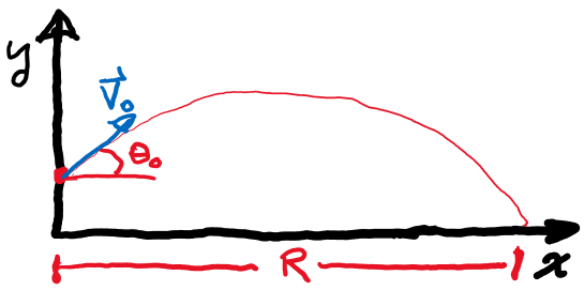
Using information from the problem statement, we can specify given information.
\[ x_0 = 0 \]
\[ y_0 = 1\ldotp 2\left[\text{m}\right] \]
\[ v_0 = 40.0\left[\text{m/s}\right] \]
\[ \theta_0 = 20\text{°} \tag{1}\]
\[ v_{0x} = v_0\cos \left(\theta_0\right) = 40.0\left[\text{m/s}\right]\cos \left(20\text{°}\right) = 37.5\left[\text{m/s}\right] \]
\[ v_{0y} = v_0\sin \left(\theta_0\right) = 40.0\left[\text{m/s}\right]\sin \left(20\text{°}\right) = 13.7\left[\text{m/s}\right] \]
As part of our analysis, we can describe physics laws that might be applicable.
Kinematic Equations for Constant Acceleration:
\[ x = x_0 + v_{0x}t \tag{2}\]
\[ y = y_0 + v_{0y}t- \frac{1}{2}gt^2 \tag{3}\]
The solution to the problem will be the value of R, which is the value of \(x\) when \(y=0\).
Design: We can express the plan for calculating R:
Put the knowns into Equation 2 and Equation 3
Solve Equation 3 for \(t\) when \(y=0\). Call this time \(T\).
Substitute the value of \(T\) obtained into Equation 2 and calculate \(x\).
Implementation: The Design plan requires some algebra, which can be done by using the quadratic formula on Equation 3. The result is
\[T = 2.88\left[\text{s}\right]\Rightarrow R = 108\left[\text{m}\right]\]
Testing: For this problem solution, testing the solution involves determining whether the value we found is sensible. A distance of 108 [m] is 354 [ft], which is less than the typical distance from home plate to the stadium edge for a professional baseball stadium (~400 [ft]).
Both Implementation and Testing will look different when the problem involves developing a computer program. We will see many examples of performing these steps as we become more involved in coding.
Basic Elements of Python
We will be using the Python programming language to develop our skills in computational science. Python was released in 1991 by its primary author, Guido van Rossum, who named the language after one of his favorite television shows, Monty Pythons Flying Circus, a comedy series produced by the BBC. Python has gone through many revisions since its introduction. We will use version 3.6 since the Google Colab platform currently supports it.
Here we introduce a few of the basic elements of the Python programming language that will enable us to start implementing our own programs. In particular, we will cover
- Literals
- Variables and Identifiers
- Operators
- Expressions
- Data Types
- Syntax
Extensive documentation for the Python programming language is provided online (Python Software Foundation, 2021).
Literals
One dictionary definition of the word “literal” is “taken at face value” and programming languages use a similar definition: a literal is a sequence of characters that stand for itself. We will consider numeric literals and string literals. These will form building blocks for writing code.
A numeric literal is a character sequence containing only the digits 0-9, a + or – sign, possibly a decimal point, and possibly the letter e, which will indicate scientific notation. A numeric literal with a decimal point is called a floating-point value. A numeric literal without a decimal point is called an integer value. One additional numerical literal is the complex value. It is written as the sum of the real part and imaginary part. The imaginary part is indicated using the character j. Here is an example:
c = 3.0 + 4.0j Commas are not used in numeric literals. Table 1 gives examples of numeric literals.
| Integer Values | Floating-point Values | Complex Values | Incorrect Values |
|---|---|---|---|
| 0 | 5. , 5.0, +5.0 | 2.0 + 3.0j | 1,500 |
| 10 | 15.25 | 4 – 5j | 1,500.00 |
| 25 | 15.25 | 0.56 + 1.7j | +1,500 |
| -25 | -15.25 | -6.0 + 7.0j | -1,500.00 |
A numeric literal with no + or – sign in front of it is considered positive.
Next we consider string literals, usually called “strings”. These are sequences of alphanumeric characters. String values are indicated using matching single quotes or double quotes:
‘My name is Bob’ , “My name is Bob”
Note that a blank character can be in a string value. If the string literal contains an apostrophe, then the value should be enclosed by matching double quotes.
“Bill’s Bookstore”
A string literal with no characters in it is called the empty string and is indicated with matching single quotes or double quotes enclosing no characters:
’’ or “”
Variables and Identifiers
An identifier is a sequence of characters that is used as a name for a programming element such as a function. The rules for constructing identifiers are
They may contain letters and digits but cannot begin with a digit.
They are case-sensitive.
They cannot contain quotes
The underscore ’_’ can be used but should be avoided as the first character.
Table 2 gives some examples of identifiers.
| Valid Identifiers | Invalid Identifiers | Reason |
|---|---|---|
| gravitationalforce | gravitationalForce’ | Cannot contain quotes |
| gravitationalForce | 2022_year | Cannot start with a digit |
| gravitational_force | _gravitationalForce V | alid but should be avoided |
A variable is a name assigned to a value. Python assigns a value to a variable by using the assignment operator, =.
num = 15The variable num now refers to the value 15. Whenever the variable num is used in a Python expression it will be replaced by the value 15. Consider the expression
num + 1This expression will evaluate to 16 since num actually represents the number 15.
A variable can be reassigned to a different value at different points in a program.
Keywords
A keyword is a predefined identifier that has a reserved specific use in a programming language. Keywords should not be used as a variable name or other user-defined identifier. If you try to do this then there will be a syntax error when the code is executed. Figure 2 shows what happens when you try to use the keyword ‘or’ as a variable.
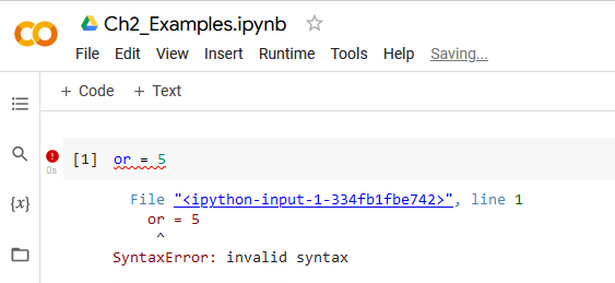
Table 3 shows all of the keyword identifiers used in Python 3.6. These identifiers are case-sensitive.
| and | del | from | None | TRUE |
|---|---|---|---|---|
| as | elif | global | nonlocal | try |
| assert | else | if | not | while |
| break | except | import | or | with |
| class | FALSE | in | pass | yield |
| continue | finally | is | raise | |
| def | for | lambda | return |
Operators
An operator is a symbol that indicates some kind of operation performed on one or more operands. An operand is a value, such as a number, that the operator acts on. Arithmetic operators such as addition, subtraction, multiplication, and division require two operands and are called binary operators. An operator that requires only one operand, such as negation, is called a unary operator.
Among the most important operators for scientific and engineering programming are the arithmetic operators shown in Table 4.
| Operator | Operation | Example | Result |
|---|---|---|---|
| -x | negation | -100 | -100 |
| x + y | addition | 100 + 25 | 125 |
| x - y | subtraction | 100 - 25 | 75 |
| x * y | multiplication | 100 * 4 | 400 |
| x / y | division | 100 / 4 | 25 |
| x // y | truncating division | 100 // 3 | 33 |
| x ** y | exponentiation | 10 ** 3 | 1000 |
| x % y | modulus | 50 % 6 | 2 |
Notice that unlike in many programming languages, exponentiation uses the operator ** rather than the caret symbol ^.
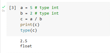
There will be times when programming requires knowing what data type is produced by an operator. Consider division using the / operator. It will always produce a float, even if both operands are integers, as shown in Figure 3.
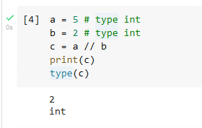
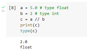
Now consider truncating division performed by the operator //. If both operands are integers (type int) then the result is an integer. If either operator is a float then the result is a float. Figure 1.6 illustrates this behavior with code snippets.
The modulus operator % may be less familiar than the other arithmetic operators. It is a binary operator that returns the remainder after performing division. If the operands are both integers (type int) then result will be an integer, otherwise the result will be a float.
Table 5 shows the cyclic nature of the modulus operator.
| Operation | Result |
|---|---|
| 0 % 5 | 0 |
| 1 % 5 | 1 |
| 2 % 5 | 2 |
| 3 % 5 | 3 |
| 4 % 5 | 4 |
| 5 % 5 | 0 |
| 6 % 5 | 1 |
| 7 % 5 | 2 |
| 8 % 5 | 3 |
| 9 % 5 | 4 |
| 10 % 5 | 0 |
Expressions
An expression is a combination of variables, values, and operators that evaluates to a single value. A sub-expression is an expression that is part of a larger expression. We will consider arithmetic expressions here. The following are examples of arithmetic expressions in Python.
\[1 + 2,3*n + 1,4*\left(n - 1\right)\]
In these expressions, the variable \(n\) must have been assigned a value, otherwise, an error will occur.
To avoid ambiguity about the order in which operators are executed in an expression, Python defines a particular order in which operators are applied. Table 6 gives the operator precedence used by Python.
| Operator | Operation | Associativity |
|---|---|---|
| ** | exponentiation | right-to-left |
| - | negation | left-to-right |
| * , / , // , % | mult , division, trunc, div, modulo | left-to-right |
| + , - | addition , subtraction | left-to-right |
The operator associativity refers to the order in which operators are applied when they have the same precedence. Consider the expression
\[4**3**2\]
Which exponentiation gets evaluated first: \(4**3\) or \(3**2\)? The right-to-left associativity rule for exponentiation says the \(3**2\) operation is performed first.
\[4**3**2\rightarrow 262144\text{ not 4096}\]
If the operator precedence in this situation had been left-to-right then the result of evaluating this expression would have been 4096.
Now consider the expression \[2/3*4\]
Since the / and * operators have the same precedence we use the left-to-right associativity rule to perform
\[2/ 3\rightarrow 0.6666\text{ then }0.6666*4\rightarrow 2.6667\]
yielding the final value 2.6667.
A good practice in coding expressions is to use parentheses to enforce a desired precedence rather than relying on the Python-defined precedence rules. Sub-expressions defined by parentheses are evaluated first.
Data Types
The formal definition of data type is a set of literal values, such as numbers or strings, and the operators that can be applied to them, such as addition and subtraction. Python uses several built-in data types. These are shown in Table 7.
| Category | Associated Python Keyword |
|---|---|
| Text Type: | str |
| Numeric Types: | int, float, complex |
| Sequence Types: | list, tuple, range |
| Mapping Type: | dict |
| Set Types: | set, frozenset |
| Boolean Type: | bool |
| Binary Types: | bytes, bytearray, memoryview |
| None Type: | NoneType |
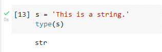
For now, we will focus only on the text and numeric types. Understanding data types can help us avoid problematic operations. For example, division, /, does not apply to strings or mixed string and numeric expressions. The following code will produce an error:
s1 = 'This is a string.'
s2 = 'This is another string.'
s1/s2 # This expression will produce an error.
Similarly
s1 = 'This is a string.'
s1/2 # This expression will produce an error.
The built-in function type(v) will tell you the data type of v.
All programming languages use the concept of data type, but the implementation differs between languages. Some languages such as C, C++, or Java require that the data type of a variable be declared explicitly before the variable can be used in an expression. This is called static typing. Other languages, including Python, will assign the data type to a variable automatically when the program is executed based on the value referred to by the variable. This is called dynamic typing. The same variable name can be assigned a different data type at different places in the program.
A complex expression can have sub-expressions or variables of different data types. These are called mixed-type expressions. In order for a mixed-type expression to evaluate to a single value, all the components or operands in the expression must be converted to a single type. This procedure can be done automatically by the Python interpreter, called coercion, or the programmer can explicitly perform conversions using data type conversion functions, which is called type conversion.
When the Python interpreter performs coercion, it will do so in a way to avoid loss of information. For example in the expression
1 + 2.5 converting the 1 to 1.0 (int to float) does not result in loss of information but converting 2.5 to 2 (float to int) does. Therefore, the int to float conversion will be done and the final value, 3.5, will be a float. We can perform the type conversions explicitly using type conversion functions. In the above example, explicit type conversion could be done with
\[\text{float}\left(\text{1}\right) + 2.5\rightarrow 1.0 + 2.5\rightarrow 3.5\]
| Type Conversion | Result |
| float(5) | 5 |
| float(‘5’) | 5 |
| float(‘A String’) | error |
| int(5.0) | 5 |
| int(5.2) | 5 |
| int(‘5’) | 5 |
| int(‘5.2’) | error |
Syntax
Syntax refers to the structure of a program and the rules about that structure. All languages have syntax. When discussing human languages such as English, syntax refers to the rules of grammar. We will introduce Python syntax rules as we learn about new elements of the language. The Python interpreter will determine if code has syntax errors and will inform you with an error message. Code that is syntactically correct can still generate a runtime error. For example
10/0
is syntactically correct but will generate an error when the expression is evaluated.
A semantic error occurs when the program is syntactically correct and generates no runtime errors, but the output is still incorrect. This means that the programmer has not translated the design of the problem solution into code correctly. Semantic errors will be the most difficult ones to eliminate.
Basic Input and Output
When we execute a program interactively, such as in a Jupyter notebook or IPython console, obtaining information from the user and communicating messages to the user will be necessary. The Python built-in functions input and print are simple methods to perform these tasks.
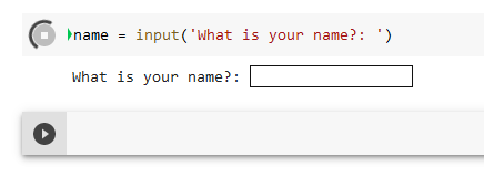
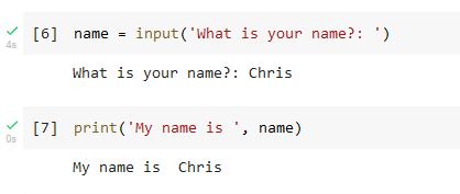
The input function will request information from the user by printing a message and then waiting for the user to enter something using the keyboard. After hitting enter or return the string entered by the user is returned to the program. For example
name = input('What is your name?:') will print the string given as the argument of the function, then wait until the user types in something, and then returns what was typed as a string that gets assigned to the variable name. Figure 7 shows how this input request looks in a Jupyter notebook.
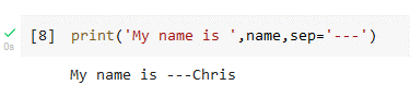
Basic output is achieved with the print function. It will print items in its argument list to the standard output, which will be an output cell in a Jupyter or Colab notebook. Multiple items can be printed by including them as comma separated items in the function argument list. Figure 8 shows an example of this behavior.
The separator between arguments printed out can be specified using the sep keyword argument. The default value is the empty string.
If the program needs to obtain a number from the user using the input function then the string that is returned will need to be converted into the appropriate numerical data type using the corresponding type conversion function. The following shows how to obtain a floating point number from the user.
float_number = float ( input ( 'Submit a floating point number:') ) After execution the variable float_number will contain the number submitted and it will be of type float.
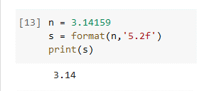
Formatting the printed output of a program can be an important part of the solution. We will discuss here one method for formatting numbers to a specified precision. We will use the built-in format function. Consider the following number.
n = 3.14159
Suppose we want to print n out with 2 decimal places. We can do this with the format function, which has the following syntax:
format(value, format_specifier) where
format_specifier: ‘[width][.precision]type’
width – total number of characters in the field
precision – number of decimal places
type –
f – float
e – exponential
Note that the width and precision fields are optional, which is indicated with the brackets.
To format the variable n to two decimal places, use the following code.
Exercises
1. The Polya general problem solving model is reformulated for computational problems to consist of the following four steps (select the correct ones):
- Analysis
- Design
- Implementation
- Testing
- Debugging
- Flowcharting
2. Which of the following are correctly formulated numerical literals?
- 1,200
- 1200
- 1200.0
3. Which of the following are legal Python variable names?
- 3CPO
- n1
- ‘number’
- chiefExecutive
- for
4. What value will the following expression have?
3 + 8 * (3**2 - 8) / 10
- 3.0
- 3
- 3.8
- 4
5. What is the value produced by each of the following expressions?
- 12/5
- 12./5.
- 12.0//5.0
- 12%5
6. What is the data type of the variable n after the following code has been executed?
n = 2
n = n*3
n = n/3
7. What is the data type of the variable num after the following statement is executed?
num = input('Type in a floating point number: ') - int
- float
- str
Program Modification Problems
1. The code presented below will request that the user submit a temperature in Fahrenheit and then converts it to a temperature in Celsius and prints out the result.
"""
Program: Temperature Conversion Program (Fahrenheit to Celsius)
Author: C.D. Wentworth
Version: 1.25.2020.1
Summary: This program will convert a temperature entered in Fahrenheit
         to the equivalent temperature in Celsius

"""

# get temperature in Fahrenheit
TF = float(input('Enter degrees Fahrenheit: '))

# calc degrees Celsius
TC = (TF - 32) * 5 / 9

# output degrees Celsius
print(TF, 'degrees Fahrenheit equals',
       format(TC, '.1f'), 'degrees Celsius')
Revise the program to do the following:
Print out a program greeting that describes what the program will do.
Requests that the user submit a temperature in Celsius.
Prints out the temperature in Fahrenheit with an appropriate message.
2. Create a program that requests a temperature from the user in Fahrenheit and then prints out the temperature in Celsius and Kelvins with appropriate messages. You can start with the code from Program Modification Problem 1.
References
Polya, G. (1971). How to Solve It: A New Aspect of Mathematical Method (2nd ed.). Princeton University Press.
Python Software Foundation. (2021). Python 3.6.15 Documentation. https://docs.python.org/3.6/
Comment Statements
Comment statements are added to code to help humans better understand what is happening in the program. Comment statements are ignored by the Python interpreter, yet they remain an important part of documenting the code. There are two methods of inserting comments:
Single line comment.
Comment Block
A single line comment is indicated with the # character. Everything after the # on the line is ignored.
A comment block is created with triple single quotes or triple double quotes. All lines between a triple single quote or double quote are ignored until another triple single quote or double quote is encountered.
Single quote block:
Double quote block: