Lists
Motivating Problem: Identifying Patterns in Global Surface Temperature Data
Climate science generates large amounts of data, including temperature and solar irradiance at specific locations on the earth’s surface over many years and time series of greenhouse gas concentrations in the atmosphere. Identifying patterns in the data is one of the important challenges for climate scientists. In this chapter, we will develop some of the computational science skills that will help with this challenge.
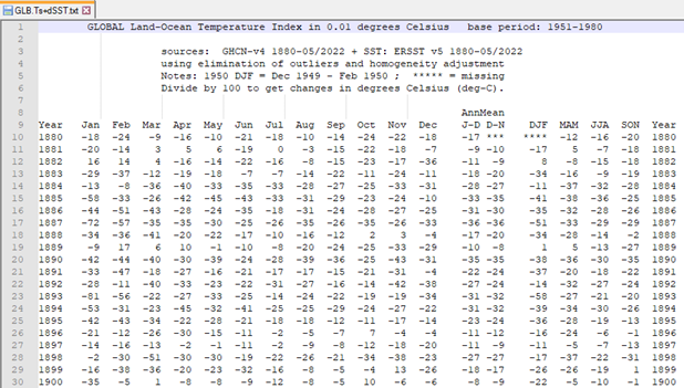
Consider one crucial climate observation: the average surface temperature of the earth. Table 1 shows some of the surface temperature data produced by the NASA Goddard Institute for Space Studies Surface Temperature Analysis group (GISTEMP Team, 2022a). The complete data set covers the years 1880-2021.
| Year | Jan | Feb | Mar | Apr | May | Jun | Jul | Aug | Sep | Oct | Nov | Dec | Ann J-D | Ann D-N | DJF | MAM | JJA | SON | Year |
|---|---|---|---|---|---|---|---|---|---|---|---|---|---|---|---|---|---|---|---|
| 1880 | -18 | -24 | -9 | -16 | -10 | -21 | -18 | -10 | -14 | -24 | -22 | -18 | -17 | *** | **** | -12 | -16 | -20 | 1880 |
| 1881 | -20 | -14 | 3 | 5 | 6 | -19 | 0 | -3 | -15 | -22 | -18 | -7 | -9 | -10 | -17 | 5 | -7 | -18 | 1881 |
| 1882 | 16 | 14 | 4 | -16 | -14 | -22 | -16 | -8 | -15 | -23 | -17 | -36 | -11 | -9 | 8 | -8 | -15 | -18 | 1882 |
| 1883 | -29 | -37 | -12 | -19 | -18 | -7 | -7 | -14 | -22 | -11 | -24 | -11 | -18 | -20 | -34 | -16 | -9 | -19 | 1883 |
| 1884 | -13 | -8 | -36 | -40 | -33 | -35 | -33 | -28 | -27 | -25 | -33 | -31 | -28 | -27 | -11 | -37 | -32 | -28 | 1884 |
| 1885 | -58 | -33 | -26 | -42 | -45 | -43 | -33 | -31 | -29 | -23 | -24 | -10 | -33 | -35 | -41 | -38 | -36 | -25 | 1885 |
| 1886 | -44 | -51 | -43 | -28 | -24 | -35 | -18 | -31 | -24 | -28 | -27 | -25 | -31 | -30 | -35 | -32 | -28 | -26 | 1886 |
| 1887 | -72 | -57 | -35 | -35 | -30 | -25 | -26 | -35 | -26 | -35 | -26 | -33 | -36 | -36 | -51 | -33 | -29 | -29 | 1887 |
| 1888 | -34 | -36 | -41 | -20 | -22 | -17 | -10 | -16 | -12 | 2 | 3 | -4 | -17 | -20 | -34 | -28 | -14 | -2 | 1888 |
| 1889 | -9 | 17 | 6 | 10 | -1 | -10 | -8 | -20 | -24 | -25 | -33 | -29 | -10 | -8 | 1 | 5 | -13 | -27 | 1889 |
| 1890 | -42 | -44 | -40 | -30 | -39 | -24 | -28 | -39 | -36 | -25 | -43 | -31 | -35 | -35 | -38 | -36 | -30 | -35 | 1890 |
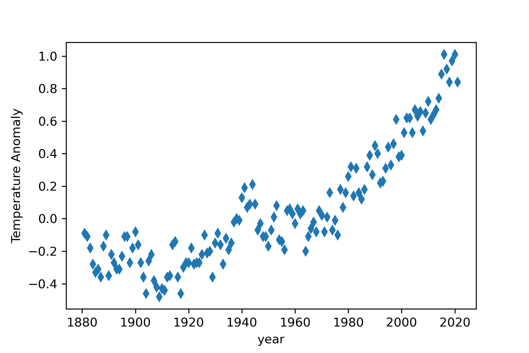
If you look at the entire 1800-2021 data table and try to identify patterns, you will likely be challenged, but a simple scatter graph of the annual mean quickly shows an interesting pattern, as seen in Figure 1.
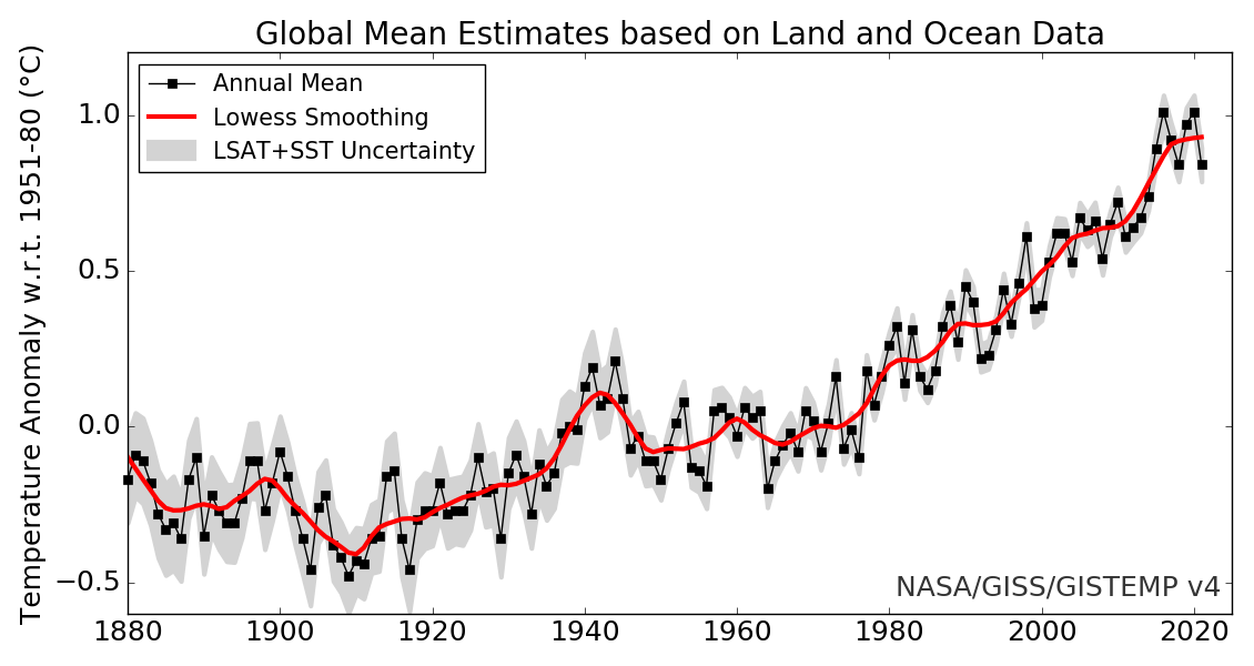
With the help of concepts developed in this chapter, the problem we must solve is how to create a graph, as shown in Figure 4.1, using tables of numerical data such as that in Table 4.1. Solving this problem will require understanding the sequence data type, reading data from a text file, and the basic use of a plotting library. We will learn about the specific examples of sequences in Python, including lists and numpy arrays. We will briefly introduce the Matplotlib plotting library used extensively for Python-based scientific visualizations.
General Properties of Lists
Lists are found frequently in everyday life: grocery lists, to-do lists, and life goals for the year. Science and engineering work also requires the use of lists. The yearly global surface temperature data introduced in Table 1 can be represented as a list. Work in genetics often requires knowing the sequence of nucleotides in a molecule of DNA, and such a sequence can be thought of as a list.
Work with lists computationally will be expedited by having an appropriate data structure representing the list structure. Python uses several such data structures. We will discuss these structures by first introducing the sequence idea, which can be considered a general definition of a list. A sequence is a linearly ordered set of values, each of which can be accessed using an index number. Table 2 gives an example of a sequence. The first value, -33, is indexed by 0 since Python uses a zero-based indexing method. Some programming languages would start indexing with the numeral 1, but not Python. This is a crucial point to keep in mind as you work with sequence data structures in Python.
| index | Value |
|---|---|
| 0 | -33 |
| 1 | -12 |
| 2 | 4 |
| 3 | -37 |
| 4 | -19 |
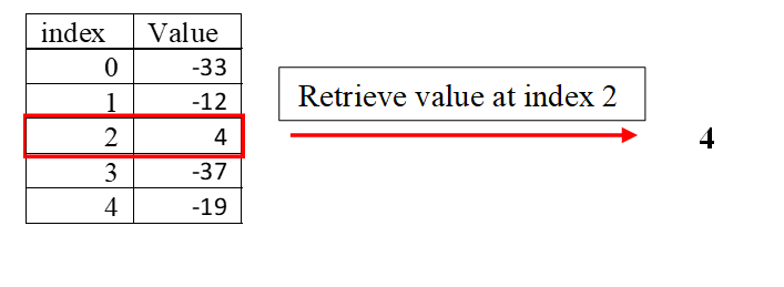
Several operations can be performed on most sequence data structures. These operations include retrieving, updating, inserting, removing, and appending an element in the sequence. Figure 2 illustrates the retrieve operation. The original sequence remains unchanged.
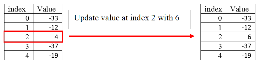
Updating a sequence value changes the value stored at a particular location. The original value is lost, and the sequence keeps the same length. Figure 3 illustrates this operation.
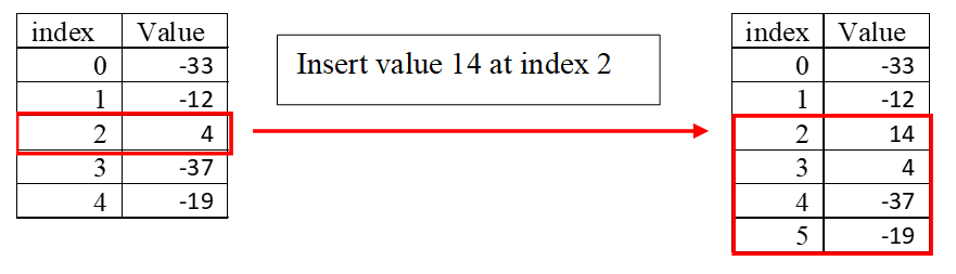
The insert operation places a new value at a particular position specified by the index but shifts all other values down. No values are lost, but the sequence increases in length. Figure 4 illustrates this effect.
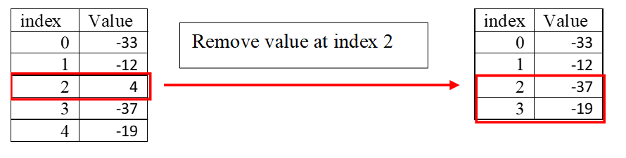
The remove operation takes out the value at a specific index and then shifts all the following up in the sequence, as shown in Figure 5.
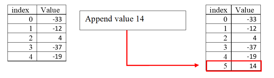
The append operation attaches a new value to the end of the sequence, as shown in Figure 6.
Sequences can be categorized as mutable, meaning that they can be changed, or immutable, meaning that the sequence cannot be changed after being defined. An immutable sequence can only have the retrieve operation applied to it. The built-in Python sequence data types include Python lists, tuples, and strings.
Python Lists
Python features a built-in sequence data structure called a list. A Python list is a mutable sequence, and the elements can have mixed data types. A Python list does not need to be all floats or all strings. It can contain a combination of floats, strings, and any other valid Python data type, including a Python list. A Python list is denoted using square brackets with elements separated by commas. Here are some examples of Python lists:
[50.5, 12.4, 72.5] [2, 4, 'two', 'four']An empty list is indicated using an empty pair of square brackets:
[]A Python variable name can be assigned to a list to facilitate working with it.
list_example = [10, 20, 30, 40]The syntax for accessing individual elements of a list (and other sequence types) is to use the index operator [] (not the same as the empty list) with an expression representing an index number inside the brackets.

Remember that Python uses zero-based indexing, so the first element of a sequence is referenced with 0. Negative index values reference elements from the right or bottom of the list rather than from the beginning.
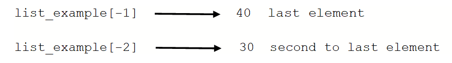
Table 3 illustrates how to perform sequence operations on a Python list.
| Operation | Example | Result |
|---|---|---|
| retrieving | list_example[2] | 30 |
| updating | list_example[1] = 50 | [10, 50, 30, 40] |
| inserting | list_example.insert(2,50) | [10, 20, 50, 30, 40] |
| removing | del list_example[1] | [10,30,40] |
| appending | list_example.append(50) | [10, 20, 30, 40, 50] |
The dot notation used in the list insert and list append operations is an example of object-oriented programming and will be explained more fully in Chapter 11. For now, think of the name to the right of the dot, called a method in object-oriented programming, as a function that applies to the object to the left of the dot.
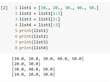
The slice operation allows us to extract multiple list elements with one simple expression. The general form is a variation of the bracket notation, [m:n], which returns elements starting with the one indexed by m and extending up to, but not including, the element indexed by n. The second through the third elements of list_example could be extracted with list_example[1:3]. If the first index number, m, is omitted, then the slice begins with the first element of the list. If the last index number, n, is omitted, then the slice includes all elements through the last one. Figure 7 illustrates the use of the slice operation.
One more common operation frequently performed on a sequence, including Python lists, is traversal. Traversing a sequence involves accessing each element in order. A simple way to do this is with a for loop. For example, printing out each element of a list on a separate line we can be done as follows:
for e in list_example:
    print(e)
Python tuples
A tuple is an immutable Python sequence data type. Tuples are defined using parentheses ().
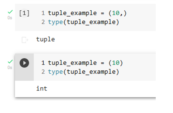
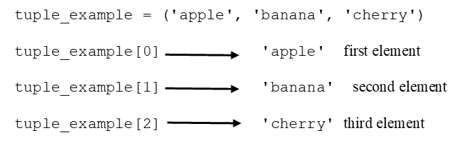
(10, 20, 30) ('apple' , 'banana' , 'cherry')To avoid ambiguity, a tuple with a single element must contain the final comma.
tuple_example = (10,)In this example, if tuple_example did not contain the final comma, then the Python interpreter would assume it is an integer. This is shown in the Colab notebook segment below.
The index syntax applies to tuples, just as it did for lists.
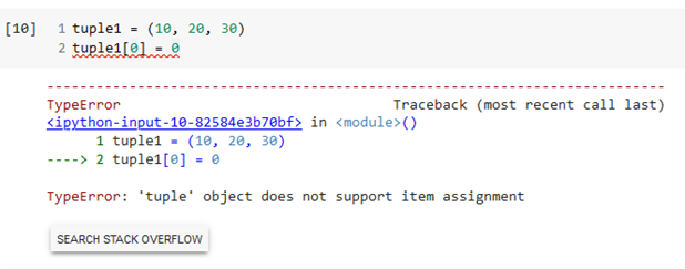
Remember that a tuple is immutable, meaning it cannot be changed after it is defined. Attempting to change a tuple element will result in an error, as shown in the notebook output below.
Python strings are an immutable sequence type, similar to tuples in behavior. The characters in a string are sequence elements, so they can be accessed using the bracket syntax.
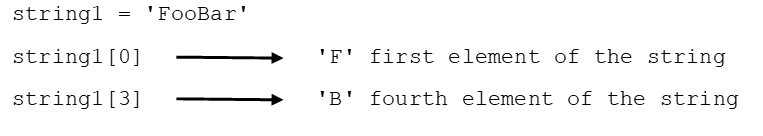
Being immutable, any attempt to reassign a character in a string will result in an error.
NumPy Arrays
The NumPy library is a crucial building block for developing Python applications for scientific and engineering computing (Numpy, 2022). This library introduces an enhanced data structure for representing multidimensional arrays, methods of operating on these arrays, and many functions that can manipulate or extract information from these arrays. The NumPy library will be used in much of the code developed in the remainder of this book. Figure 9 illustrates the structure of arrays. A one-dimensional array is a type of sequence that behaves similarly to vectors in linear algebra. Two-dimensional arrays can be considered as matrices, and higher-dimensional arrays can be considered tensors, as understood in certain areas of mathematics, such as differential geometry, engineering, and physics.
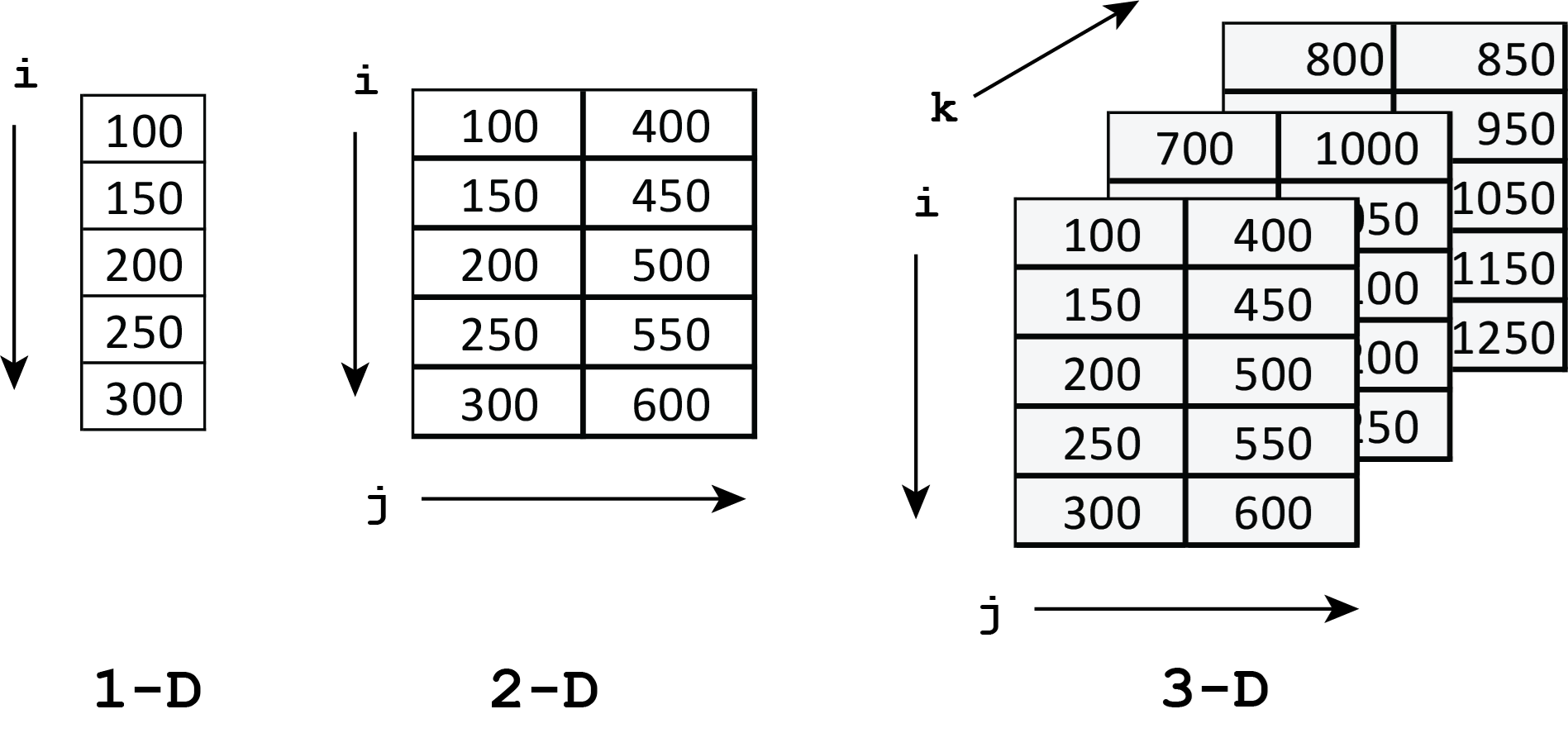
The array data structure or array object introduced by NumPy is called a ndarray, which stands for an n-dimensional array. The elements of a ndarray must all be of the same data type, called the dtype, such as integer or float. Two significant properties are associated with a specific ndarray: the array elements shape and the data type (dtype). The shape of a ndarray is a tuple that specifies the size of the array along each dimension.
We will start with one-dimensional arrays to develop our understanding of NumPy arrays and operations on them. One way to create a NumPy array is to use the array routine in NumPy.
import numpy as np
a = np.array([10., 20., 30, 40.], dtype='float64')
Before using NumPy arrays and operations on them, we must first import the NumPy package. Renaming the package ‘np,’ while unnecessary, has become traditional in data science applications. The first argument of the array routine is a Python list. The second argument specifies the data type of the elements in the array. The shape and data type of a NumPy array can be obtained as follows.
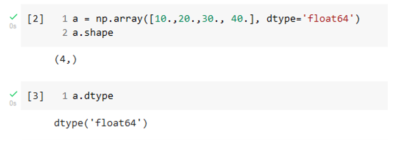
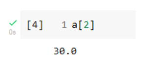
Note that the shape is given as a tuple and shows that a is a one-dimensional array with four elements. The individual values in a NumPy array can be retrieved using the square bracket notation.
Now let us move on to a two-dimensional NumPy array.
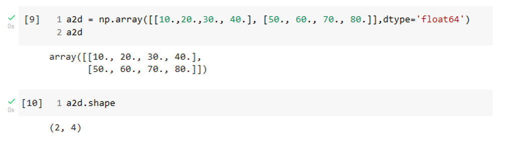
The shape of a2d indicates that there are two dimensions. The first value in the shape tuple gives the number of rows, and the second value gives the number of columns. We can retrieve the value of individual elements in the array using square bracket notation. For example, the element in the second row and fourth column can be accessed as follows.
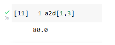
The first index number gives the row, and the second index number provides the column. Recall that Python uses a zero-based indexing system.
One advantage of using NumPy arrays instead of Python lists is that numerical calculations can be coded more succinctly. Suppose we have an array of numbers, and we need to add a constant value to each array member. This can be done with one line of code if the array is represented in a NumPy array.
a1d = np.array({[}10., 20., 30.{]})
b1d = a1d + 5.0
If a1d were a Python list, then the arithmetic expression would yield an error. We would need to set up a loop to add the constant to each element explicitly.
Basic Input and Output with Files
A basic operation that any data-oriented computational scientist must perform is reading columns of numerical data from a file into a program for processing and then writing out columns of numerical data to a file for use at a later time. In this section, we will learn about one method of performing these operations that uses a function in the NumPy module, one that will take care of many of the tedious processes that arise in performing reading and writing numerical data.
Let’s work with a specific example. The file GLB.Ts+dSST.txt is a plain text file that contains the global mean temperature anomaly data compiled by NASA’s Goddard Institute for Space Studies Surface Temperature Analysis project, shown in Table 1. Figure 10 shows a screenshot of this file viewed with a plain text editor. We see that the file has eight lines of comments that describe the dataset, one line that specifies column headings, and then 20 columns of numbers. Spaces separate the numbers in each row, so we call this space-delimited data.
The NumPy package provides a function for importing numerical data from a text or CSV file as long as the data is in the form of columns of numbers. Since this is a common situation in scientific and engineering applications, we will use this technique here. The NumPy function we will use is loadtxt. While loadtxt can skip rows of non-numerical data at the beginning of the file, only numerical data must be present in the imported columns. The file shown in Figure 10 has missing numbers, indicated by ***, and the presence of these characters will cause an error. To use loadtxt, we must do some initial cleanup of the data file. One way to accomplish this cleanup is to open the file in a plain text editor and delete the rows that have missing numbers. The revised file is called GLB.Ts+dSST_clean.txt. Keeping the original file unchanged is a good practice in case problems arise in the data processing workflow.
The code that will read in the data and separate the year column and the annual mean temperature anomaly column is shown below.
import numpy as np

# Read in data and extract columns
cols = np.loadtxt('GLB.Ts+dSST_clean.txt', skiprows=9)
year = cols[:, 0]
annual_temp_anomaly = cols[:, 13]

# Calculate the actual annual temperature anomaly
annual_temp_anomaly = annual_temp_anomaly/100.If you are using Google Colab notebooks as your development environment, you will need to upload the data file to your Google Drive. You will then need to mount the Google Drive and change the working directory to wherever you placed your file, typically in the same folder as the Colab notebook file. This can be accomplished by adding the following code at the beginning of the Colab notebook.
from google.colab import drive
drive.mount('/content/drive')
%cd /content/drive/MyDrive/yourWorkingDirectory
You should replace ‘yourWorkingDirectory’ with the path to the folder where your data file is located on your Google Drive.
The function savetxt from the NumPy module can be used to write columns of numerical data to a text file. The first argument gives the file name to which data is written. The second argument provides the 2d numpy array containing the data columns. A delimiter can be specified with the delimiter keyword. Figure 4.13 shows the output file. By default, the format of the numbers will be scientific notation with the full precision for floats. The following code snippet, Figure 12, shows how to construct a 2d NumPy array from columns of data and then write out the data to a text file, a portion of which is shown in Figure 13.
# Create 2d array from year and temperature 1d arrays
outArray = np.column_stack((year, annual_temp_anomaly))

# Save to text file
np.savetxt('annual_temp_anomaly.txt', outArray, delimiter='\t')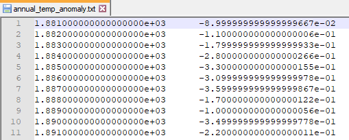
We can specify the format for the numbers written out using the fmt parameter. This parameter is a string with the following form:
%[flag]width[.precision]specifier
where each part is described below:
flags (optional):
- : left justify
+ : Forces to precede result with + or -.
0 : Left pad the number with zeros instead of space (see width).
width: The minimum number of characters to be printed. The value is not truncated if it has more characters.
precision (optional):
For integer specifiers (e.g., d, i,o,x), the minimum number of
digits.

For e, E, and f specifiers, the number of digits to print after
the decimal point.

For g and G, the maximum number of significant digits.

For s, the maximum number of characters.
specifiers:
c: character

d or i: a signed decimal integer

e or E: scientific notation with e or E.

f: decimal floating point

g, G: use the shorter of e, E or f

o: signed octal

s: a string of characters

u: an unsigned decimal integer

x, X: unsigned hexadecimal integer
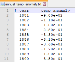
The fmt parameter can be a single format specifier, which will be applied to all the columns of numbers, or it can be a list of format specifiers, one for each column. Since the first column of the output is supposed to be a year, it would be more natural to format that number as an integer. This can be accomplished with the following statement.
# Save to text file
header_string = 'year\t temp anomaly'
np.savetxt('annual_temp_anomaly.txt', outArray, fmt=['%6i','%10.2e'],
           delimiter='\t', header=header_string)
A header that gives column labels is provided with the header keyword argument. A portion of the output file is shown in Figure 14.
Introduction to Scientific Visualization with Matplotlib
We are ready to create our first scientific visualization: a two-dimensional scatter graph showing the relationship between the mean global temperature anomaly and year. There are several standard plotting packages available in Python, but we will focus on Matplotlib since it is widely used and forms the basis for other visualization packages (The Matplotlib Development team, 2021) . We will discuss scientific visualizations in greater detail in Chapter 5. Here, we want to touch on the basics of using the Matplotlib package to create a 2d scatter graph.
Let us assume that the mean global surface temperature anomaly values and corresponding year are in the data file annual_temp_anomaly.txt. The following code produces a simple scatter graph of this data.
import numpy as np
import matplotlib.pyplot as plt

# Read in data
cols = np.loadtxt('annual_temp_anomaly.txt',skiprows=1)
year_data = cols[:,0]
temp_anomaly_data = cols[:,1]

# Plot data
plt.plot(year_data, temp_anomaly_data, linestyle='', marker='d', markersize=5.0)
plt.xlabel('year')
plt.ylabel('Temperature Anomaly')
plt.savefig('tempAnomalyVsYear.png', dpi=300)
plt.show()
The pyplot sub-package of the Matplotlib package is imported and renamed plt. This is traditional in data science applications. The entire Matplotlib package is not needed to create most of the plots we use. The plot is created with the Matplotlib plot function. The first argument is the 1d array containing the x-axis values. The second argument is the 1d array with the y-axis values. The other keyword arguments are set, so only data points are graphed with a diamond data marker. The markersize is always adjusted to achieve a good visualization. Axis labels are added with the xlabel and ylabel functions.
Finally, the plot is saved as a graphics file with the savefig function. The graphics file format is determined from the extension on the chosen file name, given as the first argument. The dpi keyword sets the resolution. The show function is not needed if the code is executed in a Jupyter notebook but will be required if it is executed in other programming environments. The plot is shown in Figure 15.
We will discuss additional methods of customizing plots in later chapters.
Computational Problem Solution: Identifying Patterns in Global Surface Temperature Data
We will now return to the problem introduced at the beginning of the chapter: how to use data visualization to help identify temperature anomaly trends over time.
Analysis
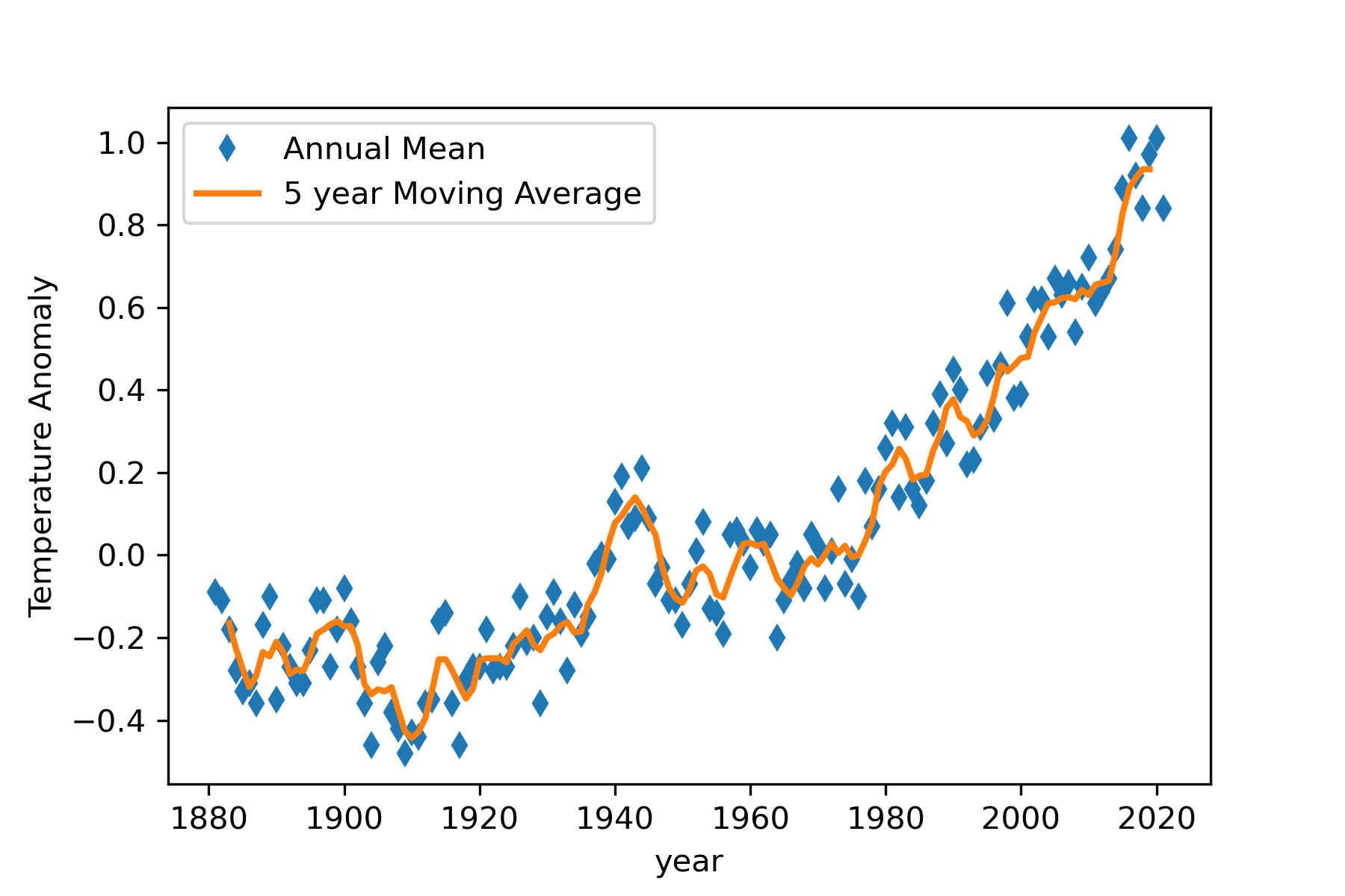
We start with a precise description of the problem and some features of the solution that will allow us to recognize a successful solution. The problem is to start with the data file given by NASA, GLB.Ts+dSST.txt (GISTEMP Team, 2022b), and produce a graph, similar to Figure 4.1, that performs some kind of smoothing of the widely fluctuating temperature anomaly values. We can recognize a solution when the graph has a smoothing curve displayed that shows fewer yearly fluctuations compared to the annual raw data.
Some quite sophisticated statistical methods exist for smoothing random fluctuating time series data, including the LOWESS smoothing shown in Figure 1. Using such techniques requires considerably more mathematical sophistication than we want to use here. Therefore, we will use a simple moving average method that is conceptually simple and relatively easy to implement computationally.
Consider a subset of the annual mean temperature anomaly data from Figure 14, shown in Table 4.
| year | temperature anomaly [C] |
|---|---|
| 1883 | -0.18 |
| 1884 | -0.28 |
| 1885 | -0.33 |
| 1886 | -0.31 |
| 1887 | -0.36 |
The 5-year moving average for the 1885 temperature anomaly is calculated from
\[T_m\left(1885\right) = \frac{\left(- 0.18- 0.28- 0.33- 0.31- 0.36\right)}{5.0}\left[\text{C}\right] = - 0.29\left[\text{C}\right] \tag{1}\]
We would replace the 1885 temperature anomaly in the data set with this new value. The moving average for each year is calculated similarly. We move the 5-year window, two years before the chosen year, two years after the selected year, plus the chosen year, to each year in turn. If \(T\left(y\right)\) represents the mean temperature anomaly for year y, then the general formula for the 5-year moving average is
\[T_m\left(y\right) = \frac{T\left(y- 2\right) + T\left(y- 1\right) + T\left(y\right) + T\left(y + 1\right) + T\left(y + 2\right)}{5} \tag{2}\]
We could try different window sizes, 7-year, 9-year, and so on, to find one that clarifies a trend, but we will stick with the 5-year window for this solution.
Design
The workflow for our problem solution is
Clean up the raw NASA data file GLB.Ts+dSST.txt so that it does not contain non-numerical data, except for the header comments.
Note the first year for which a 5-year moving average can be calculated (defines first_year).
Note the last year for which a 5-year moving average can be calculated (defines last_year).
Write code to import the year and annual mean columns from the clean data file.
Convert the annual mean column numbers to Celsius by dividing them by 100.
Write code that can calculate the 5-year moving average temperature anomaly for a general specified year, named current_year.
Step 1 is performed with a basic text editor application, and we assume that the cleaned-up data file is GLB.Ts+dSST_clean.txt.
For the NASA data set we are using here, the first year for which a 5-year moving average can be calculated is 1883, and the last year is 2019.
Steps 4 and 5 were discussed in section 4.5. These steps define the year_data and annual_temp_anomaly arrays.
Step 6 requires some thought. Assume that year_index is the index number giving the year currently being considered. To expedite using the Matplotlib plot function, we will also define two new 1d NumPy arrays: moving_year_data will contain all the years for which we calculate a moving average, and moving_annual_temp_anomaly will contain the corresponding calculated moving averages. A pseudocode snippet of this process is shown below.
Extract the subset of temperature anomalies from annual_temp_anomaly
  (this defines anomaly_subset)
Calculate the mean of the numbers in anomaly_subset (defines
   temp_anomaly_mean)
Add the temp_anomaly_mean to moving_annual_temp_anomaly
All of the variables required for the problem solution are listed in Table 5.
| Data Structure | Type | Description |
|---|---|---|
| first_year | float variable | first year for the 5-year moving average calculation |
| last_year | float variable | last year for the 5-year moving average calculation |
| year_data | 1-d numpy array | contains the column of year values in the NASA data set |
| annual_temp_anomaly | 1-d numpy array | contains the column of annual temperature anomaly values in the NASA data set |
| year_index | integer variable | specifies the year currently being calculated |
| anomaly_subset | 1-d numpy array | contains the five temperature anomalies that will be averaged |
| moving_year_data | 1-d numpy array | contains the year values for which a moving average is calculated |
| moving_annual_temp_anomaly | 1-d numpy array | contains the moving average value for each year in moving_year_data |
Implementation
We can collect together pieces of code from sections 4.5 and 4.6 to create code for our problem solution. Since NumPy arrays do not allow for the append operation, as can be done with a Python list, we must create new NumPy arrays with the correct length before using them. An empty array is created using the NumPy empty function, as shown below in lines 29 and 30.
The subset of the temperature anomaly values to be averaged is obtained from an array slicing operation in line 36. The average of the subset values is obtained using the NumPy mean function in line 37.
"""
Title: 5-year Moving Average Plot
Author: C.D. Wentworth
Version: 6.29.2022.1
Summary: This program will read in annual temperature anomaly data
         provided by NASA, calculate a 5-year
         moving average, then plot both the raw data and moving average.
Revision History:
    6.29.2022.1: base

"""
import numpy as np
import matplotlib.pyplot as plt

cols = np.loadtxt('GLB.Ts+dSST_clean.txt', skiprows=9)
year_data = cols[:, 0]
annual_temp_anomaly = cols[:, 13]

# Calculate the actual annual temperature anomaly
annual_temp_anomaly = annual_temp_anomaly/100.

# Define the year range
first_year = 1883.
last_year = 2019.
first_year_index = np.where(year_data == first_year)[0][0]
last_year_index = np.where(year_data == last_year)[0][0]

# Create empty numpy arrays for plot
moving_year_data = np.empty(len(year_data)-4)
moving_annual_temp_anomaly = np.empty(len(moving_year_data))

# Calculate the moving average
moving_year_index = 0
for year_index in range(first_year_index, last_year_index + 1):
    # obtain temperature anomaly subset
    anomaly_subset = annual_temp_anomaly[year_index - 2:year_index + 2]
    temp_anomaly_mean = np.mean(anomaly_subset)
    moving_year_data[moving_year_index] = year_data[year_index]
    moving_annual_temp_anomaly[moving_year_index] = temp_anomaly_mean
    moving_year_index = moving_year_index + 1
The code block that creates the plot is shown below. The linestyle keyword argument is used to choose whether a line is solid, dotted, or dashed. The empty string, , indicates no line is drawn, which is often used when plotting data points. The linestyle value - indicates a solid line. The label keyword argument specifies a string that is used when a legend is shown. The legend is produced with default placement by
plt.legend()We will discuss keyword arguments used in the plot function in greater detail in the next chapter. Generally, a review of examples from the Matplotlib documentation or tutorials can help figure out good choices for the keyword argument values (The Matplotlib Development Team, 2022) .
# plot the raw data and moving average
plt.plot(year_data, annual_temp_anomaly, linestyle='', marker='d',
         markersize=5.0, label='Annual Mean')
plt.plot(moving_year_data, moving_annual_temp_anomaly, linestyle='-',
         linewidth=2, label='5 year Moving Average')
plt.xlabel('year')
plt.ylabel('Temperature Anomaly')
plt.legend()
plt.savefig('tempAnomalyVsYearMovingAvg.png', dpi=300)
plt.show()
The complete listing is contained in the chapter program file 5_year_moving_average_plot.py.
Testing
When the 5-year Moving Average Plot program is executed, we get the graph shown in Figure 16. This plot does resemble the one produced by NASA scientists, shown in Figure 1. This provides evidence that the problem solution is correct. The five year moving average line shows more fluctuations than the LOWESS smoothing line in Figure 1. This is likely due to the five year moving window being smaller than that used in the LOWESS smoothing algorithm. It would be interesting to compare a seven year moving average with the five year moving average.
Exercises
1. (Fill-in-the-blank): A sequence is a ________ ordered set of values, each of which can be accessed using an _____ number
- Which of the following Python data structures are mutable? Choose all that apply.
- lists
- strings
- tuples
- NumPy arrays
3. What is the resulting list when the value at index three is removed?
| index | value |
|---|---|
| 0 | 25 |
| 1 | 15 |
| 2 | -5 |
| 3 | 50 |
| 4 | 75 |
a.
|
b.
|
||||||||||||||||||||||
c.
|
d.
|
4. What are the index values for a tuple with 4 elements?
- 0-4
- 0-3
- 1-4
5. How would you define a tuple with the one element 12?
- [12]
- [12,]
- (12,)
6. What would be the list resulting from the [1:3] slice in
[80, 70, 75, 50, 65]
- [80, 70, 75]
- [70, 75, 50]
- [70, 75]
7. Select all true statements about Python sequence data types.
- All items in a Python list must be the same data type (all integers, all strings, etc.).
- An attempt to assign a new value to a tuple element will result in an error.
- Python lists, tuples, and strings all use zero-based indexing.
- Write a Python expression that prints out the third element of list1 defined below.
list1 = [125, -75, 25, 50, 15]
Program Modification Problems
1. In this exercise, you are given a program, shown below, that generates a list of random numbers and then counts the number of odd numbers in the list. You need to modify the program so that it creates two lists of random numbers, adds up the odd numbers in one list, adds up the even numbers in the second list, and then adds the two sums together.
"""
Program: Count Odds
Author: C.D. Wentworth
Version: 2.5.2020.1
Summary: This program creates a list of random numbers and
         counts how many odd numbers are in the list.

"""
import random as rn

# make a list of random numbers
lst = []
for i in range(10):
    lst.append(rn.randint(0, 1000))

# count the number of odd numbers in the list
odd = 0
for e in lst:
   if e % 2 != 0:
       odd = odd + 1
print('The number of odd numbers in the list is: ',odd)
2. The program below will create a tan(t) graph. Modify it to create a plot of the following function
\[f\left(t\right) = 5.0 \ast \sin \left(t\right)\]
for \(- 3.14 \leq t \leq 3.14\).
The plot should have
a dashed red line with a thickness of 5.
The x-axis title should be ‘t.’
The y-axis title should be ‘f(t).’
The y-axis scale should be adjusted to \(- 6 \leq t \leq 6\)
The chart title should be ‘5*sin(t) versus t’. The font size should be 20. The font color should be green.
"""
Program: Plot Function
Author:
Version: 1.25.2020.1
Summary: This script creates a basic plot of a function with
         user chosen features including the line style and
         line width.

"""

import matplotlib.pyplot as plt
import numpy as np
x = np.linspace(-3,3,100)
y = np.tan(x)
plt.plot(x,y,color='g',linestyle='-',linewidth=4)
plt.xlabel('x',fontsize=16)
plt.ylabel('y',fontsize=16)
plt.title('tan(x) vs x',fontsize=24, color='red')
plt.grid(True)
plt.axis(ymin=-10,ymax=10)
plt.show()
3. Write a program that creates a plot of \(\cos \left(t\right)\) and \(\sin \left(t\right)\) for \(0 \leq t \leq 2\pi\) with both plots on the same graph. You can start with the Chapter 4 Program Modification Problem 2 code. Your final graph should
show sin as a solid red curve
show cos as a solid blue curve
have a legend
show the title ‘Comparison of cos and sin’ in green.
use \(- 1.5 \leq y \leq 1.5\) for the y-axis scale
Program Development Problems
1. Write a program that will create a moving average plot of the NASA global temperature anomaly data for a user specified moving average window. The user will specify a window size that should be an odd number of years. The program should calculate the required moving average for as many years in the data as possible and then create a plot of the annual data, shown with data symbols, and the moving average, shown as a solid line.
References
GISTEMP Team. (2022a). Data.GISS: GISS Surface Temperature Analysis (v4): Analysis Graphs and Plots. https://data.giss.nasa.gov/gistemp/graphs/
GISTEMP Team. (2022b). GISS Surface Temperature Analysis (GISTEMP), version 4. [Database]. NASA Goddard Institute for Space Studies. https://data.giss.nasa.gov/gistemp/
NumPy. (2022). https://numpy.org/
The Matplotlib Development team. (2021). Matplotlib—Visualization with Python. https://matplotlib.org/
The Matplotlib Development Team. (2022). Tutorials—Matplotlib 3.5.2 documentation. https://matplotlib.org/stable/tutorials/index.html