Fitting Models to Data: The Method of Least Squares
Motivating Problem: Damped Spring {
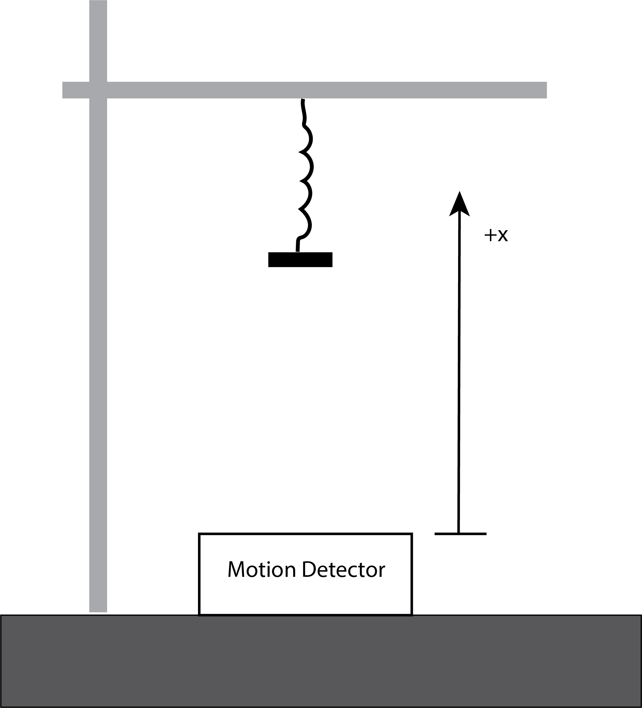
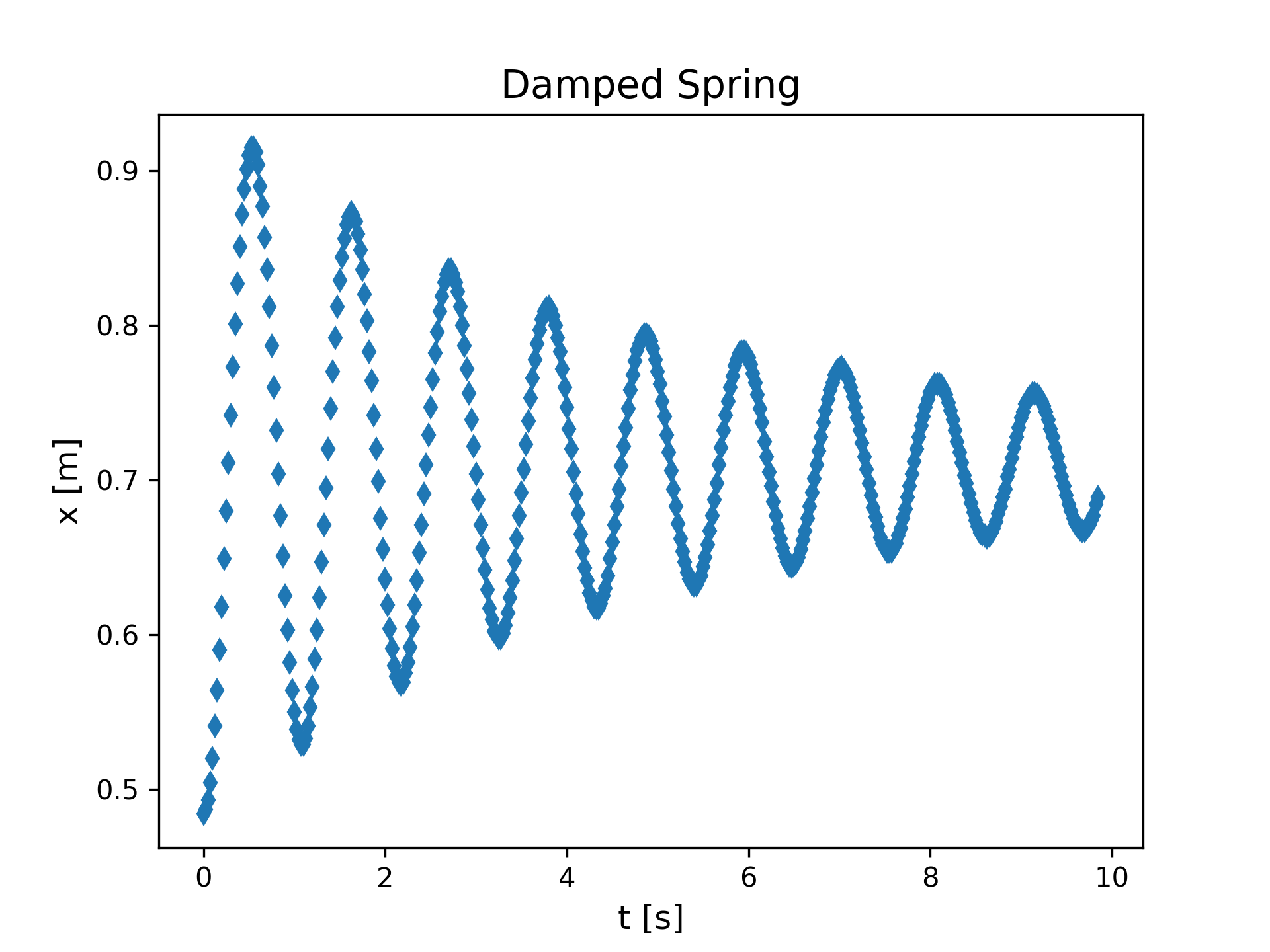
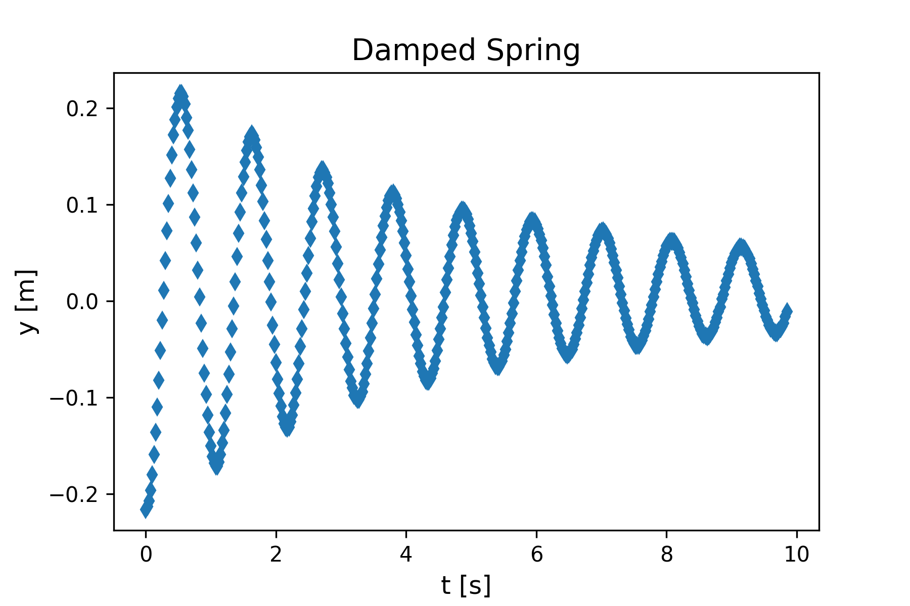
Figure 1 shows the setup for a physics experiment involving a mass m (= 0.550 [kg]) attached to a spring. The spring is stretched from rest and released. Position data collected by a motion detector is shown in Figure 2. Since the data shows significant damping, the situation will require more than simply the ideal force law (Hooke’s Law: \(F=-ky\)) to understand. By adding a drag force proportional to velocity, \(-bv_y\), an appropriate model can be constructed. The solution to Newton’s 2nd Law is discussed in most general physics textbooks and yields (Knight, 2016)
\[\begin{array}{l} y\left(t\right) = Ae^{- bt/ 2m}\cos \left(\omega t + \phi_0\right) \\ \\ \omega = \sqrt{\omega_0^2- \frac{b^2}{4m^2}}\text{ , }\omega_0 = \sqrt{\frac{k}{m}} \\ \end{array} \tag{1}\]
In Equation Equation 1, \(y(t)\) is the position measured with respect to the mass’s equilibrium position.
|
|
Our computational problem will be to choose the best-fit values for the model parameters, A, b, and k, so that the model equation fits the provided data.
Introduction
In Chapter 7 on dynamical systems, we considered a mathematical model for the growth of bacteria. Our development of the model was guided by some actual data on growth for a couple of different species of bacteria. When we needed to choose values for parameters that appeared in the model, we used a trial-and-error method to choose values that gave a good fit of the model to the available data. We need a more statistically sophisticated method that can choose best-fit values and estimate how much experimental uncertainty the values have.
The Method of Least Squares
Definition
While there are several methods that can be used to statistically estimate best-fit model parameter values, we will use the method of least squares. It is a widely used method and usually a good first-choice for the models we often encounter in science and engineering. We will introduce the basic framework with some formal definitions and then move on to implementing the method computationally, first with simple linear models and then with more complex non-linear models.
Let us assume that we have a model with independent variables \(\mathbf x = \left(x_1,x_2,\ldots ,x_v\right)\), a set of model parameters \(\mathbf p = \left(p_1,p_2,\ldots ,p_m\right)\), and the model function \(f\left(\mathbf x;\mathbf p\right)\) that determines the dependent variable y.
\[y = f\left(\mathbf x;\mathbf p\right) \tag{2}\]
In the simplest case there will be just one independent variable, but the method works for more complex cases.
Suppose we have performed an experiment that produced n data points
\[\left(\mathbf x_1,y_1\right),\ldots ,\left(\mathbf x_n,y_n\right)\]
Next, we define a function called the Least Square Estimator, \(L\left(\textbf{p}\right)\), by the equation
\[L\left(\mathbf p\right) = \sum_{i = 1}^n\left(y_i- f\left(\mathbf x_i;\mathbf p\right)\right)^2 \tag{3}\]
Note that L is a function of the model parameters. The least squares method for data fitting involves choosing the model parameter values p that minimize the function L.
Linear Regression
If we are using a simple linear model
\[y=ax+b \tag{4}\]
then statisticians have derived closed-form formulae for the best-fit slope, a, and intercept, b. They use the calculus principle that necessary conditions for a function to be a minimum are that first partial derivatives with respect to the independent variables must be zero. This is symbolized by
\[\begin{array}{left} \frac{\partial L\left(a,b\right)}{\partial a} = 0 \\ \frac{\partial L\left(a,b\right)}{\partial b} = 0 \\ \end{array} \tag{5}\]
These equations can be solved for the best-fit values of a and b. We will not work through the calculus or give the explicit formulae. You will learn to do that in a more advanced statistics course (Akritas, 2018). Instead, we will learn how to implement the linear least squares technique numerically, letting the computer do all of the work.
We will use a specific example to learn this technique. Consider a rigid container with some air in it. We measure the pressure of this gas as the temperature is varied. The volume is held constant. Figure 3 shows some of the data from the file GasData.txt.
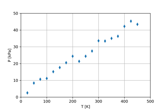
Visual inspection of the figure suggests that a linear model should fit this data rather well. We will use the method of least squares, linear regression version, to find the best fit slope and intercept. We expect the data presented in Figure 3 to fit the following model equation:
\[P=aT+b \tag{6}\]
Minimizing the Least Squares Estimator function involves minimizing the vertical distance between the data points and the theoretical model value. Consider Figure 4, which shows our data with a linear model drawn as a red line.
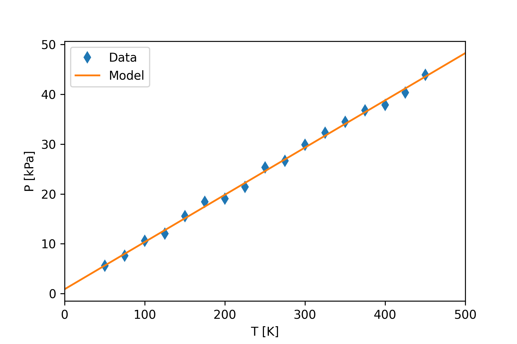
The method of least-squares will find the model parameters, the slope and intercept in this case, that will minimize the sum of the squares of the residuals. The model line shown in Figure 4 was produced by the linear regression formulae from the least squares method. It is hard to imagine a different line that would come closer to the data points.
We will make use of a Python library function that will apply the linear regression formulae to the data set and give the user the optimized slope and intercept. The function is from the scipy.stats library. It is the scipy.stats.linregress() function (The SciPy Community, 2022b).
Syntax:
out = scipy.stats.linregress(x,y)x = a list with the independent variable values
y = a list with corresponding dependent variable values
The function returns a list-like data structure, called out above, containing the following values (data type in parentheses)
slope : (float) slope of the regression line
intercept : (float) intercept of the regression line
r-value : (float) correlation coefficient
p-value : (float) two-sided p-value for a hypothesis test whose null hypothesis is that the slope is zero.
stderr : (float) Standard error of the slope estimate
The following lines of code will retrieve all of these values from the variable out.
slope = out[0]
intercept = out[1]
rvalue = out[2]
pvalue = out[3]
se = out[4]
Figure 5 shows a Python script that will apply the linregress function to the gas data. The code produces the following text output.
slope= 0.0948
intercept= 0.8803
rvalue= 0.9986
pvalue= 1.32e-20
se= 0.0013
Figure 4 shows the graph produced by the code.
"""
Program: Gas Data Fit
Author: C.D. Wentworth
Version: 3-20-2017.1
Summary:
    This program reads in pressure-temperature data and fits
    the data to a linear model using the scipy.stats.linregress()
    function.
Version History:
    3-20-2017.1: Base

"""

import numpy as np
import matplotlib.pyplot as plt
import scipy.stats as ss
# import data
cols = np.loadtxt('GasData.txt',  skiprows=3)
tData = cols[:, 0]
PData = cols[:, 1]
# Fit data to linear model
out = ss.linregress(tData, PData)
slope = out[0]
intercept = out[1]
rvalue = out[2]
pvalue = out[3]
se = out[4]
print('slope= ', format(slope,'7.4f'))
print('intercept= ',format(intercept,'7.4f'))
print('rvalue= ',format(rvalue,'7.4f'))
print('pvalue= ',format(pvalue,'7.2e'))
print('se= ',format(se,'7.4f'))
# Plot the data
plt.plot(tData,PData,linestyle='',marker='d',label='Data')
plt.xlabel('T [K]')
plt.ylabel('P [kPa]')
plt.xlim((0,500))

# Plot the theory
tTheory = np.linspace(0,500,100)
PTheory = slope*tTheory + intercept
plt.plot(tTheory,PTheory,label='Model')
plt.legend()
plt.savefig('GasData.png') Non-linear Regression
Case 1: Model Function is Known Explicitly
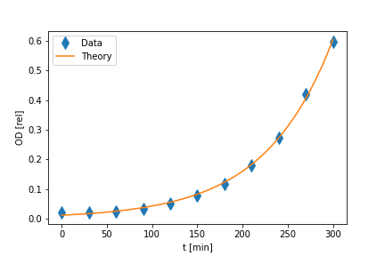
The method of least-squares can also be applied to fitting data to a non-linear model, such as the exponential growth model. Figure 6 shows the growth of bacteria.
It is clear that a linear model will not describe this data. Indeed we know that an exponential growth model should work well. Equation 7 gives the equation defining this model.
\[N\left(t\right) = N_0e^{rt} \tag{7}\]
The complication with applying the method of least-squares to a non-linear model is that we do not have explicit formulae for the model parameters, N0 and r, as we did in the linear case. The computational problem is to perform a search through the parameter space to find the values that will minimize the Least Square Estimator good starting place. We will make use of a Python library function that will search for the model parameter values that minimize the Least Squares Estimator function given an initial starting guess for the values. The function is from the scipy.optimize library. It is the scipy.optimize.curve_fit()function (The SciPy Community, 2022a). Here is the basic syntax for using the curve_fit function.
popt, pcov = scipy.optimize.curve_fit( f , tData , fData , p )f is the callable function that calculates the theoretical value for the independent variable t. It must be in the form
\(f(t, parameters)\)
where t, the independent variable must be listed first, and parameters must be listed separately, not in a tuple variable.
tData and fData are lists containing independent and dependent variable values for data points.
popt will be the list of optimized parameter values.
pcov contains the covariance matrix. It gives information about the uncertainty in the parameter estimates. Explicit values for statistical uncertainty are obtained using
psterr = np.sqrt(np.diag(pcov))psterr is a list containing the standard error of each parameter estimate in the same order as in popt.
Figure 7 shows a program that can fit the exponential growth model of Equation 7 to the data of Figure 6.
"""
Program: Non-linear Least Squares - Explicit Function Form
Author: C.D. Wentworth
Version: 10.25.2022.1
Summary: This program reads in bacterial growth data and fits
the data to the non-linear exponential growth model using the
scipy.optimize.curve_fit() function.
Version History:
  3.28.2017.1: base version
  10.25.2022.1: added parameter uncertainty calculation

"""

import numpy as np
import matplotlib.pylab as plt
import scipy.optimize as so

def N(t,N0,r):
    tmp = N0*np.exp(r*t)
    return tmp

# import data
cols = np.loadtxt('BacterialGrowthData.txt', skiprows=9)
tData = cols[:, 0]
ODData = cols[:, 1]

# Define initial guess for model parameters
N0 = 0.021
r = 0.020
p = N0,r

# Fit data to exponential growth model
popt,pcov = so.curve_fit(N, tData, ODData, p)
p_stderr = np.sqrt(np.diag(pcov))

# Plot the data
plt.plot(tData, ODData, linestyle='', marker='d',
         markersize=10.0, label='Data')

# Plot the theory
N0,r = popt
dN0 = p_stderr[0]
dr = p_stderr[1]
tTheory = np.linspace(0, 300, 50)
ODTheory = N(tTheory,N0,r)
plt.plot(tTheory, ODTheory, label='Theory')
plt.xlabel('t [min]')
plt.ylabel('OD [rel]')
plt.legend()
plt.savefig('bacterialGrowthFitData.png')

# print out best-fit model parameters
print('N0 = ', format(N0,'6.4f'), '+-', format(dN0,'7.4f'))
print('r = ', format(r,'6.4f'), '+-', format(dr,'6.4f'))
Figure 6 shows the model fit to the data. The program will produce the following printed output giving least squares fit model parameter values and uncertainties.
N0 = 0.0112 +- 0.0007
r = 0.0133 +- 0.0002
Case 2: Model Function value must be obtained by numerical integration
We have worked with mathematical models where the actual model function describing how the dependent variable depends on the independent variable is not known, but instead the model is defined by an ordinary differential equation or system of such equations. We learned how to numerically integrate the differential equation to obtain model values for selected independent variable values.
How can we use the least squares technique for finding best-fit model parameters for this case where we must integrate a differential equation to get model values? We can still use the curve_fit function to perform the least squares minimization search, but we must do some extra work to give it the required callable model function. The function will be defined to have the form
f(t, parameters)
but inside this function definition we use the numerical integration function scipy.integrate.solve_ivp and integrate the differential equation from the initial independent variable value up to the desired independent variable value. The function will return just this last calculated dependent variable value, as required by the curve_fit function.
We will continue to work with the exponential growth model as a test case for working through the details of this method. The rate equation for the population function \(y\left(t\right)\) is
\[\frac{dy}{dt} = ry\left(t\right) \tag{8}\]
and there is a known initial condition of the form
\[y\left(0\right) = y_i\]
Let’s start with the basic setup required to use solv_ivp to integrate the exponential growth rate equation that we discussed back in Chapter 7. We must define a Python function f that calculates the rate of change of the state variable y for an array of independent variable values t.
import scipy.integrate as si
import numpy as np
import matplotlib.pylab as plt
import scipy.optimize as so

# Create a function that defines the rhs of the differential equation system

def f(t,y,r):
#   y = a list that contains the system state
#   t = the time for which the right-hand-side of the system equations
#       is to be calculated.
#   r = a parameter needed for the model
#
#   Unpack the state of the system
    y0 = y[0] # value of the state variable y at t
#   Calculate the rates of change (the derivatives)
    dy0dt = r*y0
    return [dy0dt]
Next, we will define the callable model function required by curve_fit that will use the numerical integration method to calculate the value of the state variable y. We will name this function yf.
def yf(t,yi,r):
    p = r,
    yv = []
    y_0 = [yi]
    for tt in t:
        if np.abs(tt)<1.e-5:
            yvt = yi
        else:
            ta = np.linspace(0,tt,10)
            # Solve the DE
            sol = si.solve_ivp(f,(0,tt),y_0,t_eval=ta,args=p)
            yvt = sol.y[0][-1]
        yv.append(yvt)
    return yv
The callable function yf for the curve_fit function is designed to accept an array of independent variable values in the t array, which will normally be a numpy array. This requires the for loop to calculate the model function value by numerical integration for each value in t. The Python code that implements this idea is shown in Figure 8 and is contained in the file expGrowthModelNonLinRegNumSol.py.
"""
Program Name: Non-linear Least Squares -
              Numerical Integration Form
Author: C.D. Wentworth
version: 10.27.2022.1
Summary: This program reads in bacterial growth data and fits
         the data to the non-linear exponential growth model
         using the scipy.optimize.curve_fit() function. This
         version uses a numerical integration method for
         calculating values of the model function.
History:
         3.17.2020.1: base
         10.27.2022.1: changed variable names

"""

import scipy.integrate as si
import numpy as np
import matplotlib.pylab as plt
import scipy.optimize as so

# Create a function that defines the rhs of the differential equation system

def f(t,y,r):
#   y = a list that contains the system state
#   t = the time for which the right-hand-side of the system equations
#       is to be calculated.
#   r = a parameter needed for the model
#

#   Unpack the state of the system
    y0 = y[0] # value of the state variable at t

#   Calculate the rates of change (the derivatives)
    dy0dt = r*y0

    return [dy0dt]

def yf(t,yi,r):
    p = r,
    yv = []
    y_0 = [yi]
    for tt in t:
        if np.abs(tt)<1.e-5:
            yvt = yi
        else:
            ta = np.linspace(0,tt,10)
            # Solve the DE
            sol = si.solve_ivp(f,(0,tt),y_0,t_eval=ta,args=p)
            yvt = sol.y[0][-1]
        yv.append(yvt)
    return yv

# Main Program

# Read in data
cols = np.loadtxt('BacterialGrowthData.txt',skiprows=9)
td = cols[:,0]
OD = cols[:,1]

# Define initial guess for model parameters
yi = 0.022
r = 0.02
p = (yi,r)

popt,pcov = so.curve_fit(yf,td,OD,p)
p_stderr = np.sqrt(np.diag(pcov))

# Calculate theoretical values
# Define the time grid
ta = np.linspace(0,300,200)
yi,r = popt
dyi = p_stderr[0]
dr = p_stderr[1]

yTheory = yf(ta,yi,r)

# print out best-fit model parameters
print('yi = ', format(yi,'6.4f'), '+-', format(dyi,'7.4f'))
print('r = ', format(r,'6.4f'), '+-', format(dr,'6.4f'))

# Plot the solution
plt.plot(td,OD,linestyle='',marker='o',markersize=10.0,
         label='Data')
plt.plot(ta,yTheory,color='g', label='Theory')
plt.legend()
plt.xlabel('t [min]')
plt.ylabel('OD [rel]')
plt.savefig('bacterialGrowthFitDataNumInt.png', dpi=300)
plt.show()The graph and print out of the best-fit model parameters are exactly the same as were produced by the code in Figure 7, which provides evidence that the more complicated numerical integration method for calculating the model function values works for the curve_fit function.
Computational Problem Solving: Damped Spring – Best-fit Model Parameter Values
We return now to the problem of the damped spring, described at the beginning of the chapter. The experimental setup is shown in Figure 10.1 and the data is contained in the file dampedSpringData.txt.
Problem Statement: Given the position-time data shown in Figure 10.2, find the best-fit model parameters by fitting the data to the damped spring position-time model function given by Equation (10.1) reproduced here.
\[\begin{array}{l} y\left(t\right) = Ae^{- bt/ 2m}\cos \left(\omega t + \phi_0\right) \\ \\ \omega = \sqrt{\omega_0^2- \frac{b^2}{4m^2}}\text{ , }\omega_0 = \sqrt{\frac{k}{m}} \\ \end{array} \tag{9}\]
Analysis: Analyze the problem
We will not reproduce the physics analysis of the situation here, since it is covered in standard university physics textbooks (Knight, 2016). The mass of the object is assumed to be fixed at the measured value of m = 0.550 [kg]. A static force constant value of k=22.9 [N/m] is also provided with the data. This value of k will not necessarily be the best-fit value for the damped oscillator. The model parameters that must be determined are \((A,b,k)\). We will use the least squares technique to find the optimum values of these parameters. We will need to use the nonlinear version of this method available to us through the curve_fit function.
Design: Describe the data and develop algorithms
The position data shows an oscillation about a nonzero equilibrium point, but the model function we are using assumes an oscillation about y=0. We can adjust the position data by a constant amount to achieve this. Use the basic data plotting template and add the following line to adjust the position.
# Read in data
cols = np.loadtxt('dampedSpringData.txt',skiprows=3)
tData = cols[:,0]
yData = cols[:,1]

# Adjust the y values by a constant amount
yData = yData - 0.7
An adjustment value of 0.7 appears to work well, as shown in Figure 9. The adjustment is applied to all values in the array yData since it is a numpy array.
Starting guesses for the model parameters must be provided to the curve_fit function. Here are some possible values to use.
\[\begin{array}{l} \begin{array}{l} A = 0.22\left[\text{m}\right] \\ b = 1.0 \\ k = 22.9\left[\text{N/m}\right] \\ \end{array} \\ \phi_0 = \pi \left[\text{radians}\right] \\ \end{array}\]
We can reuse the algorithm design used for the code in Figure 7. We just need to replace the model function N used in that code with the model function from Equation 9 .
Implementation
The design described above implemented in Python code is shown in Figure 10. The code is in the file dampedSpringModelNonlinearRegression.py.
"""
Program: Damped Spring Model Data Fitting
Author: C.D. Wentworth
Version: 10.25.2022.1
Summary: This program reads in position-time data for
an object attached to a damped spring and fits
the data to the standard damped spring model function
using the scipy.optimize.curve_fit() function.
Version History:
  10.25.2022.1: base

"""

import numpy as np
import matplotlib.pylab as plt
import scipy.optimize as so

def yf(t, A, b, k, phi0):
    m = 0.550  # [kg]
    w0 = np.sqrt(k/m)
    w = np.sqrt(w0**2 - b**2/(4.0*m**2))
    tmp = A*np.exp(-b*t/(2.0*m))*np.cos(w*t + phi0)
    return tmp

# Read in data
cols = np.loadtxt('dampedSpringData.txt',skiprows=3)
tData = cols[:,0]
yData = cols[:,1]

# Adjust the y data values by a constant amount
yData = yData - 0.7

# Define initial guess for model parameters
A = 0.22
b = 1.0
k = 22.9
phi0 = np.pi
p = A, b, k, phi0

# Fit data to the damped spring model
popt,pcov = so.curve_fit(yf, tData, yData, p)
p_stderr = np.sqrt(np.diag(pcov))

# Plot the data
plt.plot(tData, yData, linestyle='', marker='d',
         markersize=7.0, label='Data')

# Plot the theory
A, b, k, phi0 = popt
dA = p_stderr[0]
db = p_stderr[1]
dk = p_stderr[2]
dphi0 = p_stderr[3]
tTheory = np.linspace(0, 10, 500)
yTheory = yf(tTheory, A, b, k, phi0)
plt.plot(tTheory, yTheory, color='red', linewidth=3, label='Theory')
plt.xlabel('t [s]')
plt.ylabel('y [m]')
plt.legend()
plt.title('Least Squares Fit to Damped Spring Model', fontsize=14)
plt.savefig('dampedSpringFitData.png', dpi=300)

# print out best-fit model parameters
print('A = ', format(A,'6.4f'), '+-', format(dA,'7.4f'))
print('b = ', format(b,'6.4f'), '+-', format(db,'6.4f'))
print('k = ', format(k,'6.3f'), '+-', format(dk,'6.3f'))
print('phi0 = ', format(phi0,'6.3f'), '+-', format(dphi0,'6.3f'))Testing
The code in Figure 10 produces the following print and graphical output.
A =  0.2203 +-  0.0024
b =  0.2084 +- 0.0038
k =  18.662 +-  0.023
phi0 =   3.072 +-  0.011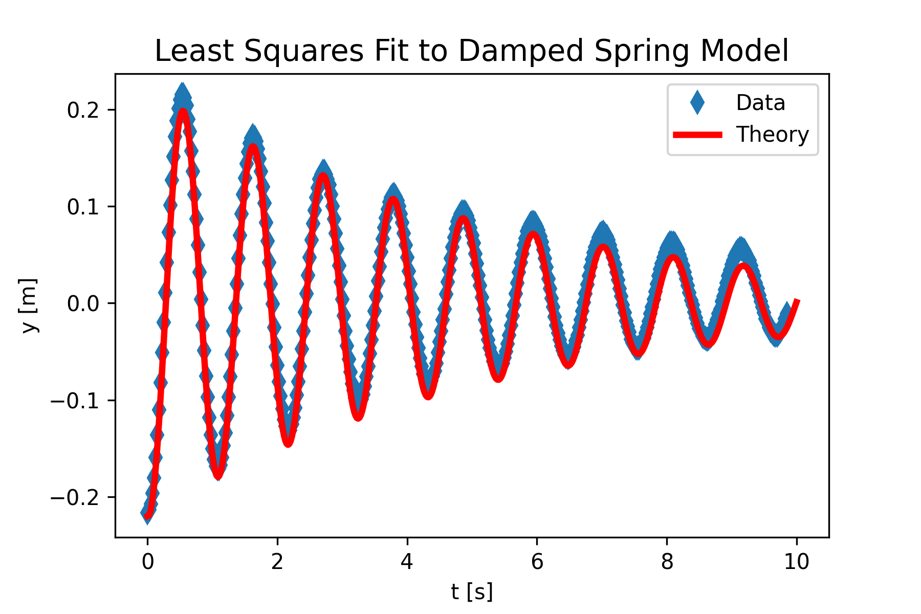
Figure 11 shows a reasonable fit between the position data and the theoretical model, although there may be some bias in the theory towards lower position values. This might be due to the constant adjustment made on the position data to yield oscillations about y = 0. This could be easily tested by adjusting the constant used in line 31.
Exercises
1. Which statements below are true for the Least Squares Method for fitting data to a model?
- It only applies to a model with one independent variable.
- It allows more than one model parameter to be estimated at a time.
- It involves minimizing the Least Squares Estimator Function.
- It can only be used to fit data to a linear model.
2. What is the calculus rule used to derive the least squares formulae for slope and intercept when fitting data to a linear model?
3. What is the name of the Python function that can perform a least squares fit of data to linear model?
4. What is the name of the Python function that can perform a least squares fit of data to nonlinear model?
Program Modification Problems
1. The Python program contained in Ch10ProgModProb1.py performs a linear regression (least-squares) fitting of some pressure versus temperature data for a gas held at constant volume. The data file for this program is GasData.txt.
The data file irisData.txt gives petal length and petal width measurements for many species of flower. You need to modify the Python code so that it performs a linear regression on this data. The program should also produce a plot of the data and the best-fit model. The graph should have
proper axis labels
a legend that shows what is the model and what is the data
major gridlines
The program should print out a message that gives
best-fit values for model parameters
standard error for the slope
the \(R^2\) value
the p-value for the fit
2. The Python program contained in Ch10ProgModProb2.py performs a non-linear regression (least-squares) fitting of bacterial growth data to the exponential model. The data file for this program is bacterialGrowthData.txt . The program fits the exponential model to the bacteria grown in Cold Spring Harbor A + 0.1% glucose (CSHA) media. The file V_natriegensGrowthData.txt contains growth data for another bacteria species. You need to modify the Python code so that it performs a non-linear regression on this data using the logistics model function. The theoretical model function is
\[y\left(t\right) = \frac{My\left(0\right)e^{rt}}{M + y\left(0\right)(e^{rt}- 1)}\]
You can use the initial OD reading for y(0), and then find the best-fit model parameters M and r. The program should also produce a plot of the data and the best-fit model. The graph should have
proper axis labels
a legend that shows what is the model and what is the data
major gridlines
The program should print out
best-fit values for the model parameters
the standard error for the model parameter estimates
3. The Python program contained in Ch10ProgModProb3.py performs a non-linear regression (least-squares) fitting of bacterial growth data to the exponential model using the numerical integration technique for obtaining the model function. The data file for this program is bacterialGrowthData.txt . The program fits the exponential model to the bacteria grown in Cold Spring Harbor A + 0.1% glucose (CSHA) media. The file V_natriegensGrowthData.txt contains growth data for another bacteria species. You need to modify the Python code so that it performs a non-linear regression on this data using the logistics model function obtained through the numerical integration technique. The theoretical rate equation is
\[\frac{dy\left(t\right)}{dt} = ry\left(1- \frac{y}{M}\right)\]
You can use the initial OD reading for y(0), and then find the best-fit model parameters M and r using the least squares technique. The program should also produce a plot of the data and the best-fit model. The graph should have
proper axis labels
a legend that shows what is the model and what is the data
major gridlines
The program should print out
best-fit values for the model parameters
the standard error for the model parameter estimates
You should get the same final results as found in the Chapter 10 Program Modification Problem 2.
Program Development Problems
1. The following video shows a physics experiment where six bundled coffee filters are dropped from rest.
The mass of the six filters is mass = 5.3 [g]. The vertical position of the filters as a function of time was obtained from the video using video analysis software. The data is contained in the file coffeeFilterData.txt.
Your task is to develop a dynamical systems model for the coffee filter motion. Go through the steps of our general problem-solving strategy. Develop the model and implement its solution in Python code. Estimate any model parameters using least squares fitting of the model to the data. Include an estimate of uncertainty in the model parameter(s). You can assume the mass of the filters and the acceleration due to gravity are already known, so the only model parameter that must be estimated is the air drag coefficient, k. An air drag force proportional to the square of the velocity will probably work well for this problem.
The position data starts at a nonzero time value. It may simplify developing the model to adjust the times to start at zero by subtracting the constant initial time from each time value.
Add a plot of the constant acceleration model (just gravity) to the figure so that a comparison can be made between the simple theory and the more complex one that includes air drag.
Create a documentation essay that describes how you went through the problem-solving strategy, detailing each step. Make sure you include a plot of the data and the best fit to the model. Specify the best-fit values of the model parameters with uncertainty.
References
Akritas, M. (2018). Chapter 6 Fitting Models to Data. In Probability & Statistics with R for Engineers and Scientists (Classic Version) (Pearson Modern Classics for Advanced Statistics Series). Pearson. http://www.librarything.com/work/17953304/book/228047240
Knight, R. (2016). Chapter 15 Oscillations. In Physics for Scientists and Engineers: A Strategic Approach with Modern Physics (4th edition). Pearson.
The SciPy Community. (2022a). scipy.optimize.curve_fit—SciPy v1.9.3 Manual. https://docs.scipy.org/doc/scipy/reference/generated/scipy.optimize.curve_fit.html
The SciPy Community. (2022b). scipy.stats.linregress—SciPy v1.9.3 Manual. https://docs.scipy.org/doc/scipy/reference/generated/scipy.stats.linregress.html