Project Ideas: Stochastic Models
Forest Fire Propagation
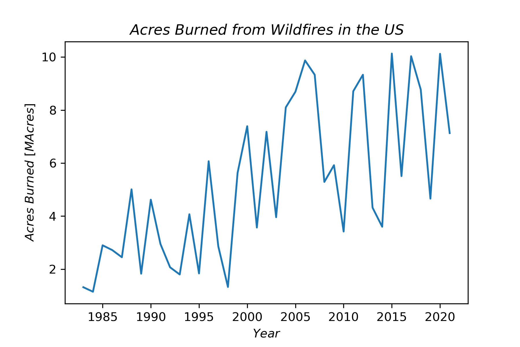
When forest fires encroach on regions with human habitation, the damage done can be substantial, including property damage, health effects, and death. Between 2017 and 2021 the average cost per year of wildfires in the U.S. was $16.8 billion, and the average number of deaths per year was 43 (Smith, 2020). If health effects of particulate inhalation are included, the death toll from wildfires climbs to about 33000 deaths per year globally (Verzoni, 2021). Figure 1 shows the acres burned by wildfires in the U.S. between 1983 and 2021, which suggests an upward trend over this time (NICC, 2022).
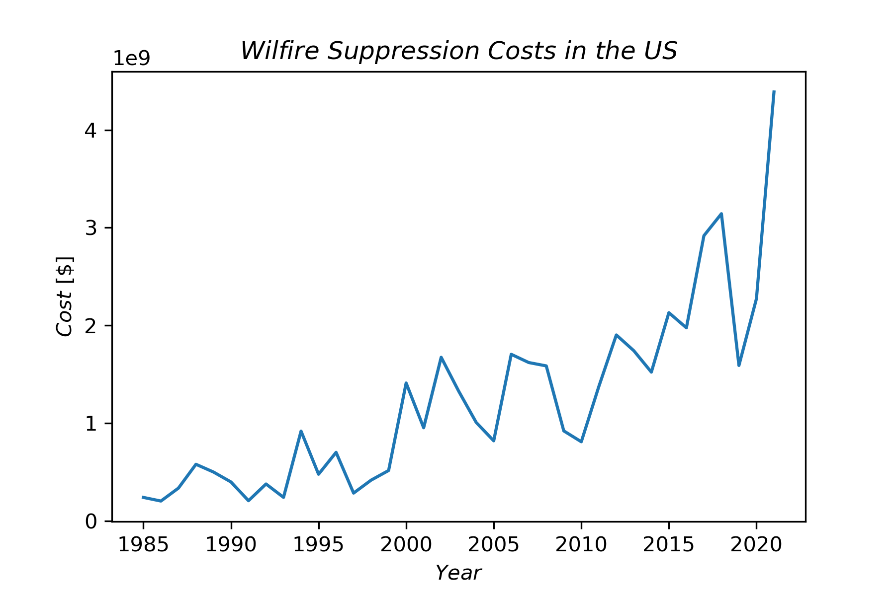
As the acres burned and human migration into forest increases, the money spent on wildfire suppression also increases, as shown in Figure 2.
The economic and health costs of wildfires have provided motivation for developing models that can help us understand and predict forest fire propagation. Historically, fire propagation models were based on partial differential equations, but more recently cellular automata models have been developed (Perry, 1998). We will explore the use of cellular automata (CA) to model forest fire propagation since the technique is mathematically and computationally simpler than using PDE’s.
Several cellular automata models for forest fires have been proposed. Some models focus on basic physics questions concerning self-organized criticality and are not meant to model real forest fires in detail (Bak et al., 1990). Other models attempt to build in features from observations of actual fires including effects of fuel moisture, wind speed, local temperature, and relative humidity (Clarke et al., 1994). More recent CA models incorporate real forest fire data to calculate the transition rules governing a cell’s change of state (Collin et al., 2011) or incorporate the effects of inhomogeneous terrain (Encinas et al., 2007).
We will outline a basic forest fire cellular automaton model. Chapter 9 gives the basic elements of a cellular automaton model. It requires
a discrete lattice of sites or cells in d dimensions, L
operating using discrete time steps
a discrete set of possible cell values, S
a defined neighborhood, N of each cell in L
a transition rule, \(\Phi\), that specifies how the state of a cell will be updated depending on its current value and the values of sites in the neighborhood.
The cellular automaton model is described by the collection \(\langle L,S,N,\Phi \rangle\).
We will develop an adaptation of the Encinas model (Encinas et al., 2007). Our model will use a 2-dimensional lattice L that can represent the earth’s surface. We will assume that L is square, with the number of grid points on one side set to a fixed value. A time step in the simulation corresponds to allowing each grid point in the lattice the chance to change state. The state of a cell is defined as
\[S_{ij} = \frac{A_{bij}}{A} \tag{1}\]
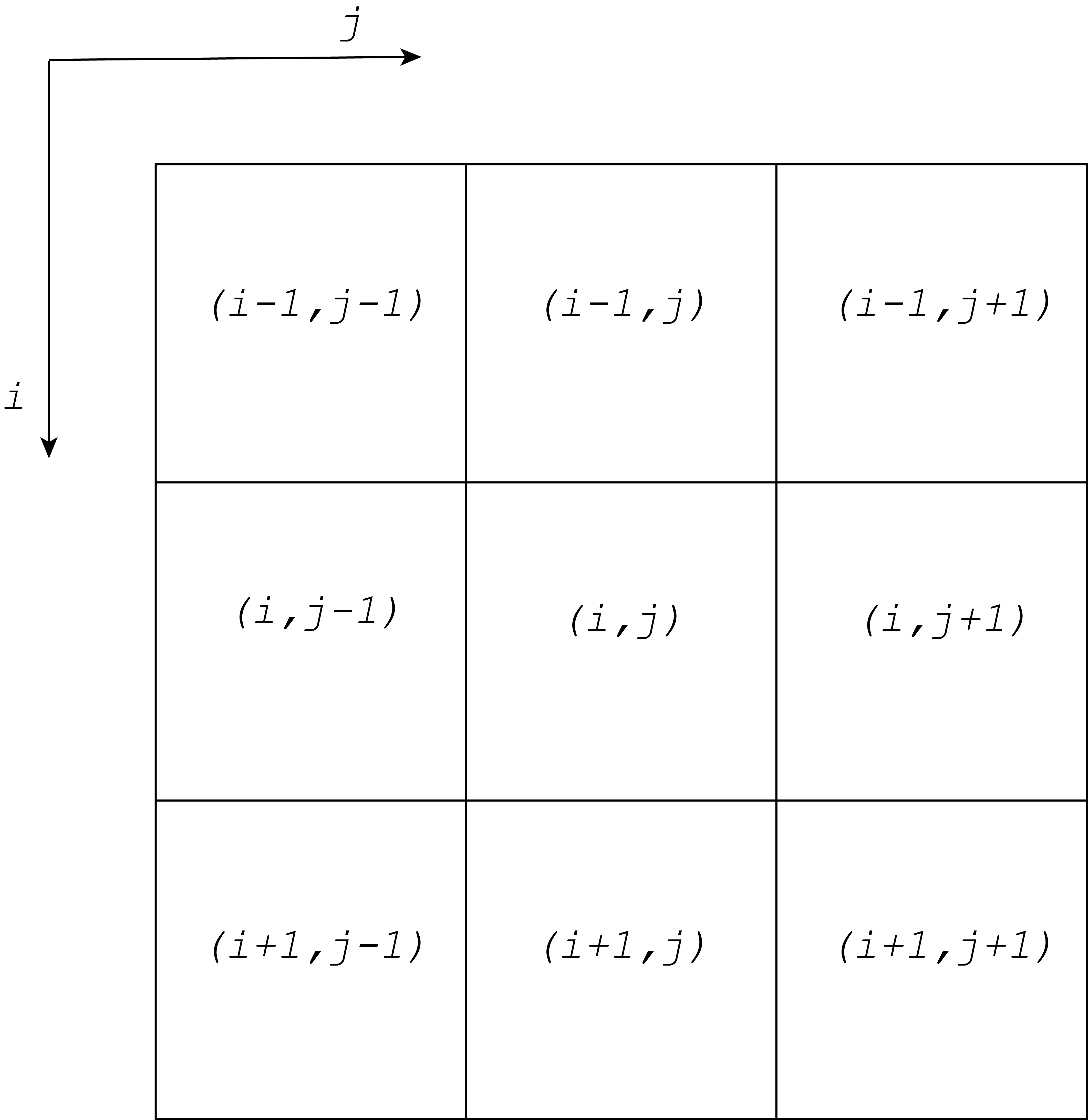
where \(A_{bij}\) is the burned area of the cell, and A is the total area of a cell. The neighborhood of a cell at (i,j) will be taken to be the Moore neighborhood illustrated in Figure 3. (Wikipedia Contributors, 2022). If (i,j) is on the lattice boundary then \(S_{ij} = 0\).
The transition rule is
\[\begin{array}{l} \Phi :S_{ij}^{(t + 1)} = \frac{R_{ij}}{R}S_{ij}^{(t)} + \sum_{(\alpha ,\beta )\varepsilon N_{adj}}\mu_{\alpha \beta}\frac{R_{i + \alpha ,j + \beta}}{R}S_{i + \alpha ,j + \beta}^{(t)} \\ \\ \quad + \sum_{(\alpha ,\beta )\varepsilon N_{diag}}\mu_{\alpha \beta}\frac{\pi (R_{i + \alpha ,j + \beta})^2}{4R^2}S_{i + \alpha ,j + \beta}^{(t)} \\ \end{array} \tag{2}\]
where \(\mu_{\alpha \beta}\) incorporates physical effects including wind speed and slope height at each cell. The values \((\alpha,\beta)\) that define the neighbors of \((i,j)\) in Equation 2 are given by
\[N_{adj} = \left\{\left(- 1,0\right),\left(0,1\right),\left(1,0\right),\left(0,- 1\right)\right\} \tag{3}\]
\[N_{diag} = \left\{\left(- 1,1\right),\left(1,1\right),\left(1,- 1\right),\left(- 1,- 1\right)\right\} \tag{4}\]
In this version of the model, we will take \(\mu_{\alpha \beta}\) to be
\[\mu_{\alpha \beta} = w_{i + \alpha ,j + \beta} \cdot h_{i + \alpha ,j + \beta} \tag{5}\]
and \(w_{i + \alpha ,j + \beta}\) are the entries in the wind speed matrix
\[W_{ij} = \left[\begin{array}{ccc} w_{i- 1,j- 1} & w_{i- 1,j} & w_{i- 1,j + 1} \\ w_{i,j- 1} & 1 & w_{i,j + 1} \\ w_{i + 1,j- 1} & w_{i + 1,j} & w_{i + 1,j + 1} \\ \end{array}\right] \tag{6}\]
and \(h_{i + \alpha ,j + \beta}\) are entries in the slope height matrix
\[H_{ij} = \left[\begin{array}{ccc} h_{i- 1,j- 1} & h_{i- 1,j} & h_{i- 1,j + 1} \\ h_{i,j- 1} & 1 & h_{i,j + 1} \\ h_{i + 1,j- 1} & h_{i + 1,j} & h_{i + 1,j + 1} \\ \end{array}\right] \tag{7}\]
If Equation 2 yields a value greater than 1 then \(S_{ij}^{\left(t + 1\right)}\) should be replaced by 1. Finally, to introduce a stochastic element into the state transition rule we assume that the cell state changes according to Equation 2 with probability p, otherwise it remains unchanged.
The state of a cellular automaton cell is usually taken to be discrete. Since Equation 2 can generally yield a continuous result, forming discrete values requires an additional step. One way to achieve state values that are discrete is to use the following definition. Assume the number of discrete values desired is Ns.
\[ S_{ij}^{\prime} = \left\{\begin{array}{left} 0 & ,S_{ij} = 0 \\ \frac{1}{\left(N_s- 1\right)} & ,0 < S_{ij} < \frac{1}{\left(N_s- 1\right)} \\ \frac{2}{\left(N_s- 1\right)} & ,\frac{1}{\left(N_s- 1\right)} \leq S_{ij} < \frac{2}{\left(N_s- 1\right)} \\ \vdots & \\ 1 & ,S_{ij} \geq 1 \\ \end{array}\right. \tag{8}\]
Some system properties that might be studied using the simulation include the percentage of cells that have not burned (Sij = 0), are burning (0<Sij <1), and have burnt out (Sij = 1) as functions of time.
Solid-State Diffusion
Diffusion is the transport of matter through the movement of individual atoms or molecules. Macroscopically, diffusion involves movement from a region of high concentration to low concentration of the diffusing material. Diffusion can be contrasted with fluid flow, where all the atoms move together due to a pressure gradient. Solid-state diffusion involves the motion of individual atoms in a solid material.
Solid-state diffusion plays a significant role in many industrial applications. Examples of materials in which solid-state diffusion plays a significant role are steel, doped semiconductors, and superionic conductors.
Steel is made from iron by the addition of carbon to iron. Uniform distribution of carbon can be achieved by diffusion of carbon atoms during a sintering process. The carbon content of solid steel can be adjusted by diffusion of carbon at the solid surface, a process called carburizing (Mandal, 2015). Other elements, such as titanium or nitrogen, can be added to iron in the same way as carbon to change the mechanical properties of the steel.
The electrical and optical properties of semiconductor materials can be adjusted by doping the base material, such as silicon, with other elements, such as gallium. This can be done by exposing the silicon to a gas containing the dopant and allowing it to diffuse into the silicon (Zant, 2014).
Superionic, or fast-ion, conductors are materials in which charge transport is achieved by moving ions rather than moving electrons, as occurs in metallic conductors (Beard, 2019). These materials are important in creating solid-state batteries, supercapacitors, and fuel cells, where solid electrolytes are required. Charge transport in these materials can be modeled by a hopping motion of ions in the solid with a preferred direction of motion established by an electric field.
We will develop a model of solid-state diffusion based on the idea of a lattice gas, in which particles that can move are placed in a lattice structure and can move between sites in the lattice. The following assumptions will be made for the model.
The diffusive motion is accomplished by a particle hopping to a nearby lattice site.
Particles can only hop to nearest-neighbor lattice sites, which are assumed to be separated by a distance a.
The particles do not interact with each other except that double occupancy of a lattice site is not allowed.
At each time step, a particle will choose a direction at random and attempt to move to the nearest-neighbor lattice site in that direction.
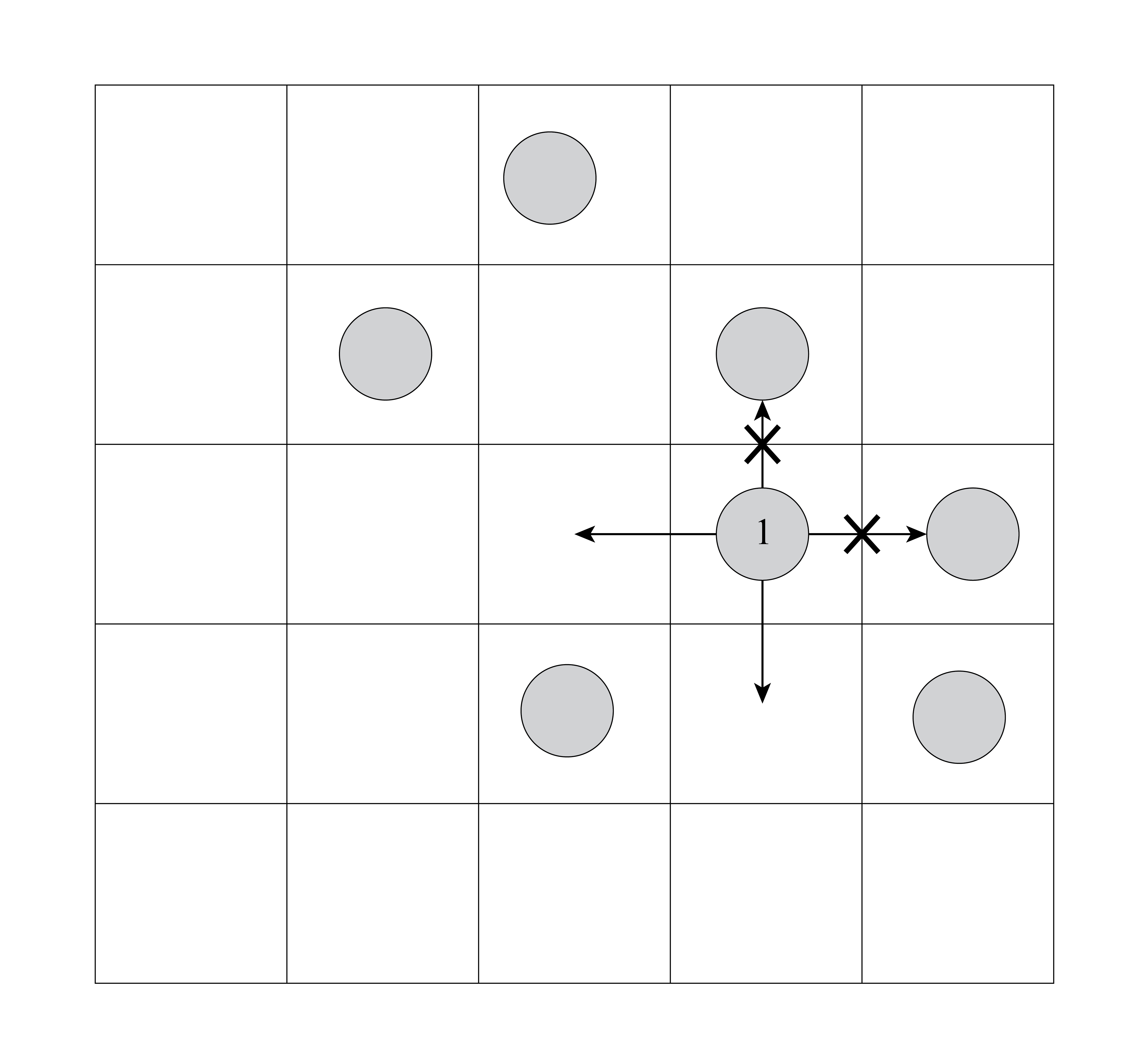
Figure 4 shows an example of a lattice gas in a two-dimensional, square lattice. The allowed nearest-neighbor hops for one particle are shown.
An important property that can be studied with this model is the tracer diffusion coefficient, D*. Tracer diffusion refers to diffusion of a single particle that can be tracked over time. The tracer diffusion coefficient can be defined in terms of the mean square displacement of the tracer particle. For the square lattice, this definition is
\[D^* = \frac{〈\left|\overrightarrow{r}\left(t\right)- \overrightarrow{r}\left(0\right)\right|^2〉}{4t} \tag{9}\]
where \(\overrightarrow{r}\left(t\right)\) is the position of the tracer at time t and the averaging, indicated by the angle brackets, is over all the diffusing particles in the lattice, since each one can be considered as a tracer.
We want to implement a Monte Carlo simulation of this model. The time t in a simulation will be considered as one pass through all the diffusing particles, attempting to allow each one to hop. The long-term time behavior of the mean square tracer displacement should be linear, giving a time-independent tracer diffusion coefficient. We can use the simulation to calculate D* as a function of particle concentration in the lattice. Table 1 defines the most important data structures or variables that might be used in the simulation code.
| Variable Name | Data Type | Description |
|---|---|---|
| concentration | float | gives the fraction of lattice sites occupied by diffusing particles |
| init_particle_positions | list | init_particle_positions[p] is a list of the initial x/y coordinates of particle number p |
| lattice_size | integer | the length of one side of the lattice as a number of sites |
| num_of_particles | integer | the number of particles in the lattice |
| p | integer | particle number |
| particle_positions | list | particle_positions[p] is a list of the current x/y coordinates of particle number p |
| site_occupancy | 2d numpy array of integers | site_occupancy[xi,yi] specifies whether the lattice site with coordinates (xi,yi) is occupied |
| t | integer | current time step being considered |
| total_time_steps | integer | the number of time steps in a simulation |
Creating Animations with Python
Animations can be used to facilitate exploring a model or data particularly when identifying time-dependent patterns. Basic animations can be created using the matplotlib package. Two methods will be discussed here.
placing the matplotlib.pyplot pause function in a for loop
using the FuncAnimation function from the matplotlib.animation package
Animations can be useful in the early stages of analyzing the models discussed in this chapter.
Using the pause() Function
The pause(interval) function from the matplotlib.pyplot package will pause program execution for the number of seconds indicated by the interval parameter. An animation can be created by setting up a for loop in which the plot function is executed and then the pause function is executed within the loop. Figure 1.5 shows an example of code that will animate plotting a function using the pause() function.
import matplotlib.pyplot as plt
import numpy as np

x = []
y = []

for i in range(100):
    x.append(i)
    y.append(np.sqrt(i))

    # Mention x and y limits to define their range
    plt.xlim(0, 100)
    plt.ylim(0, 10)

    # Ploting graph
    plt.plot(x, y, color = 'green')
    plt.pause(0.01)

plt.show()Using the FuncAnimation Function
The matplotlib.animation package has a function named FuncAnimation that requires a bit more work to set up than just using the pause function but allows for more flexibility including being able to save the animation in a gif, avi, mov, or mp4 file format. Using FuncAnimation to create an animation requires the following steps
defining an empty figure object
defining a callable Python function that can create one frame of the animation, usually performed using the matplotlib plot function
making a call to the FuncAnimation function
Defining the empty figure object is done using the Object Oriented interface for matplotlib. The basic syntax for creating an empty plotting grid is
fig = plt.figure()
axes = fig.add_subplot(1,1,1)
The callable function that creates a frame must have the frame number as the first argument with any other arguments following:
def func(frame, *fargs)where frame will be an integer specifying the frame number being created.
FuncAnimation has many parameters (The Matplotlib development team, 2023). A basic call will be of the form
animation_name = animation.FuncAnimation(fig=fig_name,
                 func=frame_creation_function, interval=time ,
                 save_count=num_of_frames)
where
fig_name is the figure object
frame_creation_function is the callable function that creates one frame in the animation
interval is the time between frames in millisecond
num_of_frames is an integer that specifies the number of frames in the animation
animation_name is a user specified variable that refers to the animation object and can be used to play the animation or save it as video file
Figure 6 gives an example of a program that produces an animation of a two-dimensional random walk.
"""
Title: Random Walk in 2D: animations
Author: C.D. Wentworth
version: 12.31.2022.1
Summary: This program performs a random walk on a
         two-dimensional lattice. It uses reflective
         boundary conditions. It produces an animation
         of the walk
version history:
        12.31.2022.1: base

"""
import random as rn
import numpy as np
import matplotlib.pyplot as plt
from matplotlib import animation
from matplotlib import rc

rc('animation', html='html5')

def createFrame(t):
    x_frame.append(x_array[t])
    y_frame.append(y_array[t])
    axes.set_title(str(t))
    plt.plot(x_frame,y_frame, scaley=True, scalex=True, linewidth=2, color="blue")


def step(xi, yi, lx, ux, ly, uy):
    import random as rn
    r = rn.randint(1, 4)
    if r == 1:
        # go east
        if xi < ux:
            xi = xi + 1
    elif r == 2:
        # go west
        if xi > lx:
            xi = xi - 1
    elif r == 3:
        # go north
        if yi < uy:
            yi = yi + 1
    else:
        # go south
        if yi > ly:
            yi = yi - 1
    return xi, yi


# --Main Program
# set up random generator
rn.seed(42)

# define the grid
lx = -30
ux = 30
ly = -30
uy = 30

# set up the simulation
N = 500
xi = 0
yi = 0
position_array = np.zeros((N + 1, 2))

# execute random walk
for i in range(1, N + 1):
    xi, yi = step(xi, yi, lx, ux, ly, uy)
    position_array[i, 0] = xi
    position_array[i, 1] = yi

x_array = position_array[:, 0]
y_array = position_array[:, 1]
x_frame = []
y_frame = []

# Create the animation
fig = plt.figure()
axes = fig.add_subplot(1,1,1)
axes.set_ylim(lx, ux)
axes.set_xlim(ly, uy)
#writervideo = animation.FFMpegWriter(fps=10)
ani = animation.FuncAnimation(fig=fig, func=createFrame, interval=100 ,
                              save_count=N)
aniThe animation object is named ani, and it is played in a Jupyter notebook by just entering the name as the last statement of the program. If you want to play the animation within an IDE such as Spyder then additional steps will usually need to be completed.
Projects
Forest Fire Propagation
Develop code that implements the model described in section 12.1. This can be done in stages, depending on available time. One way to start the fire is to initialize one cell to the state in the range \(0 < S_{ij} < 1\). Another possible initial state would be to allow a given concentration c of the cells to be burning. For each of the following scenarios, measure the percentage of cells in the burning state as a function of time. Consider the effect of varying p and c.
1. Assume a homogeneous lattice, so there is no variation in burn rates, no wind, and no variation in height. This is accomplished by
setting all entries of R to one
letting the wind and height matrices be defined by
\[W_{ij} = \left[\begin{array}{ccc} 1 & 1 & 1 \\ 1 & 1 & 1 \\ 1 & 1 & 1 \\ \end{array}\right]\text{ , }H_{ij} = \left[\begin{array}{ccc} 1 & 1 & 1 \\ 1 & 1 & 1 \\ 1 & 1 & 1 \\ \end{array}\right]\]
2. Consider an inhomogeneous system with burn rates that vary in some way on the lattice. You might consider dividing the lattice into two regions with different burn rates.
3. Explore the effect of wind speed. A north-to-south wind is represented by the wind matrix
\[W_{ij} = \left[\begin{array}{ccc} 1.5 & 1.5 & 1.5 \\ 1 & 1 & 1 \\ 0.5 & 0.5 & 0.5 \\ \end{array}\right]\]
Solid-State Diffusion
1. Implement the 2-dimensional diffusion model discussed in section 12.2. Study the mean square displacement of a particle \(〈\left|\overrightarrow{r}\left(t\right)- \overrightarrow{r}\left(0\right)\right|^2〉\) as a function of time and as a function of concentration. Does it become linear after some period of time, indicating a well-defined tracer diffusion coefficient? Does the lattice size have an effect on the results? Remember that when performing a Monte Carlo simulation of a model, measured properties of the system will show random variation. To eliminate the effects of this random variation you must repeat the simulation multiple time and form a mean over all the simulations for any measured property, as discussed in Chapter 9.
2. Develop a model for diffusion in a one-dimensional lattice similar to the two-dimensional model. Implement a Monte Carlo simulation of the model. Does the mean-square displacement \(〈\left|x\left(t\right)- x\left(0\right)\right|^2〉\) behave the same as in two dimensions?
References
Bak, P., Chen, K., & Tang, C. (1990). A forest-fire model and some thoughts on turbulence. Physics Letters A, 147(5), 297–300. https://doi.org/10.1016/0375-9601(90)90451-S
Beard, K. W. (Ed.). (2019). SECTION C: SOLID-STATE ELECTROLYTES (CERAMIC, GLASS, POLYMER). In Linden’s Handbook of Batteries (5th edition.). McGraw-Hill Education. https://www.accessengineeringlibrary.com/content/book/9781260115925/toc-chapter/chapter22/section/section24
Clarke, K. C., Brass, J. A., & Riggan, P. J. (1994). A cellular automaton model of wildfire propagation and extinction. Photogrammetric Engineering and Remote Sensing. 60(11): 1355-1367, 60(11), Article 11.
Collin, A., Bernardin, D., & Séro-Guillaume, O. (2011). A Physical-Based Cellular Automaton Model for Forest-Fire Propagation. Combustion Science and Technology, 183(4), 347–369. https://doi.org/10.1080/00102202.2010.508476
Encinas, A. H., Encinas, L. H., White, S. H., Rey, A. M. del, & Sánchez, G. R. (2007). Simulation of forest fire fronts using cellular automata. Advances in Engineering Software, 38(6), 372–378. https://doi.org/10.1016/j.advengsoft.2006.09.002
Mandal, S. K. (2015). Heat Treatment and Welding of Steels. In Steel Metallurgy: Properties, Specifications and Applications (First edition.). McGraw-Hill Education. https://www.accessengineeringlibrary.com/content/book/ 9780071844611/chapter/chapter8
NICC. (2022). Wildfires and Acres. National Interagency Fire Center. https://www.nifc.gov/fire-information/statistics/wildfires
NIFC. (2022). Suppression Costs National Interagency Fire Center. National Interagency Fire Center. https://www.nifc.gov/fire-information/statistics/suppression-costs
Perry, G. L. W. (1998). Current approaches to modelling the spread of wildland fire: A review. Progress in Physical Geography: Earth and Environment, 22(2), 222–245. https://doi.org/10.1177/030913339802200204
Smith, A. B. (2020). U.S. Billion-dollar Weather and Climate Disasters, 1980—Present (NCEI Accession 0209268) [Data set]. NOAA National Centers for Environmental Information. https://doi.org/10.25921/STKW-7W73
The Matplotlib development team. (2023). Matplotlib.animation.FuncAnimation. Matplotlib 3.6.3 Documentation. https://matplotlib.org/stable/api/_as_gen/matplotlib.animation.FuncAnimation.html
Verzoni, A. (2021). Global Wildfire Deaths. http://www.nfpa.org/News-and-Research/Publications-and-media/NFPA-Journal/2021/Winter-2021/News-and-Analysis/Dispatches/International
Wikipedia Contributors. (2022). Moore neighborhood. In Wikipedia. https://en.wikipedia.org/w/index.php?title=Moore_neighborhood&oldid=1128664897
Zant, P. V. (2014). Doping. In Microchip Fabrication (6th ed.). McGraw-Hill Education. https://www.accessengineeringlibrary.com/content/book/9780071821018/ chapter/chapter11