Project Ideas: Dynamical Systems Models
Overview
One of the best ways to develop computational science skills for creating and solving models of scientific and engineering systems is to work on substantive projects that require analysis of the problem, finding appropriate data, and then developing code by reusing elements learned in previous chapters.
In this chapter, we will focus on developing dynamical systems models of several topics in the areas of biology, engineering, and physics. For each topic, we will present some basic background, provide references for additional background, define some of the key features of a model, and then suggest questions that can be explored with a computational solution to the model.
Biology
HIV Infection of an Individual
Human Immunodeficiency Viruses (HIV) are virus species that cause Acquired Immunodeficiency Syndrome (AIDS). There are two known species of HIV, labeled HIV-1 and HIV-2, both of which can cause AIDS. HIV are retroviruses, which contain RNA that can produce the DNA required for viral reproduction once a virus particle infects a host cell. HIV infects primarily T-lymphocyte cells, although they eventually infect a wide variety of cell types in the human host (Levy, 1993).
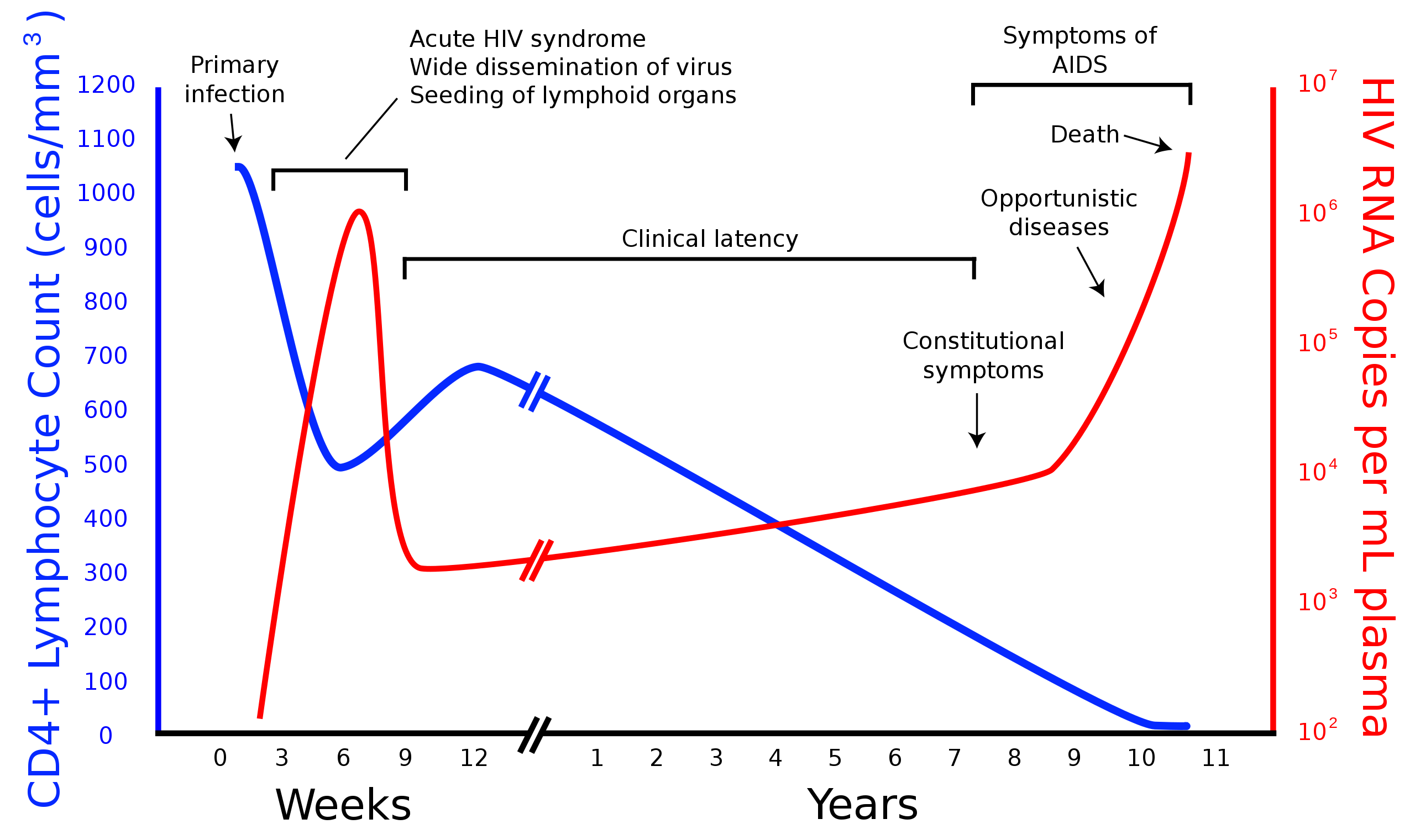
Figure 1 shows the life cycle of viral load and CD4+ Lymphocyte concentration in an individual after infection (Wikipedia Contributors, 2022). The time development of the infection can be divided into three periods: the primary (or acute) infection, the latent (or asymptotic or chronic) period, and finally the onset of AIDS. The appearance of AIDS, usually several years after HIV infection, is associated with the destruction of the immune system, as illustrated by the significant reduction in CD4+ T-cell concentration.
Mathematical modeling of HIV infection dynamics has played a critical role in understanding how AIDS develops and in aiding creation of effective antiviral treatments (Ribeiro & Perelson, 2004). In this project you will focus on developing a model of HIV dynamics during the acute stage of the infection. In particular, the model must predict the initial rapid increase in viral load and then its decrease to a stable longer term value. Additionally, the model should predict the initial rapid decrease in the uninfected CD4+ T-cell concentration and then its rise to a longer-term value that slowly decreases over time.
A good approach to this modeling problem is to use the dynamical systems framework with different compartments to represent the kind of cells and free viral particles that will be considered. The simplest compartment model that shows success at modeling the primary stage of infection is a three compartment model described by the state variables
\[\begin{array}{l} T = \text{concentration of uninfected T-cells} \\ I = \text{concentration of infected T-cells} \\ V = \text{concentration of free virus} \\ \end{array}\]
and represented by Figure 2.
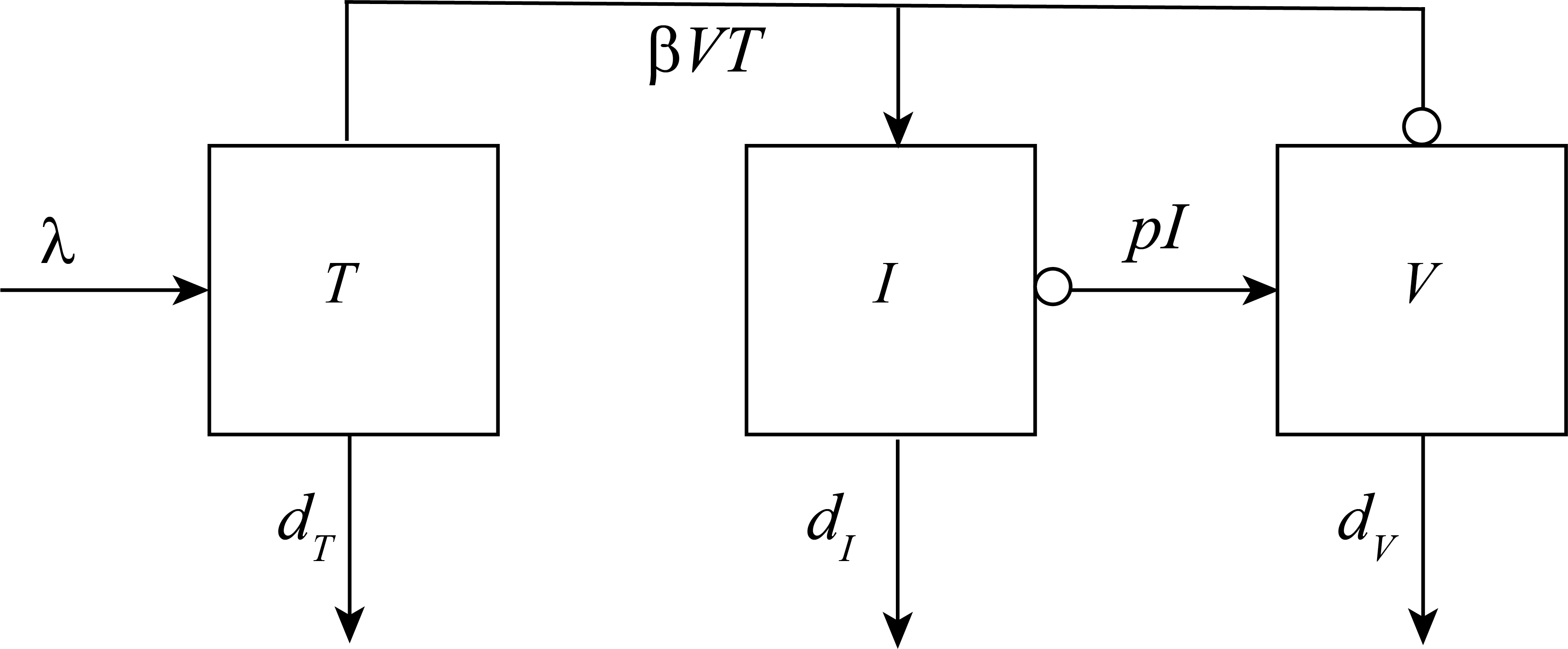
The rate equations associated with Figure 2 are (Perelson & Ribeiro, 2013)
\[\begin{array}{l} \frac{dT}{dt} = \lambda - d_TT- \beta VT \\ \\ \frac{dI}{dt} = \beta VT- d_II \\ \\ \frac{dV}{dt} = pI- d_VV \\ \end{array} \tag{1}\]
Epidemiology of the COVID-19 Infection
Epidemiology is the study of patterns in the development of a disease in a population, and is of interest to researchers in basic science and by public health policymakers. One disease that is of particular interest at the time of publication is COVID-19, a serious global pandemic that appeared at the end of 2019.
COVID-19 is a disease caused by the severe acute respiratory syndrome coronavirus 2 (SARS‑CoV‑2). There have been 651,918,402 confirmed cases and 6,656,601 deaths globally of COVID-19 since December 2019 (WHO Coronavirus (COVID-19) Dashboard, 2020). In addition to the clear health consequences, the disease triggered significant economic and political disruption throughout the world.
Mathematical models of epidemics in a population can aid exploration of basic questions about an infectious disease and offer guidance to policy makers about preparing for or responding to an epidemic. These observations are true for the study of the COVID-19 pandemic (Adiga et al., 2020). Mathematical models can help answer critical questions such as
How quickly will the disease sweep through a population?
How many people will be infected during the outbreak?
Will the disease persist in the population?
The starting point for investigating population-level dynamics of infectious diseases is the Susceptible-Infectious-Recovered (SIR) compartmental model. The state variables are
\[\begin{array}{l} S = \text{The number of susceptible people} \\ I = \text{The number of infected people} \\ R = \text{The number of recovered people} \\ \end{array}\]
The basic SIR model is represented in Figure 3. The assumptions that are used in the basic model are
There is no birth and death of people, so the total population of people is a constant.
Susceptible people will become infected through exposure to infected people.
Infected people are immediately infectious.
The rate of recovery \(\gamma\) is assumed to be constant and recovered people are immune to infection.
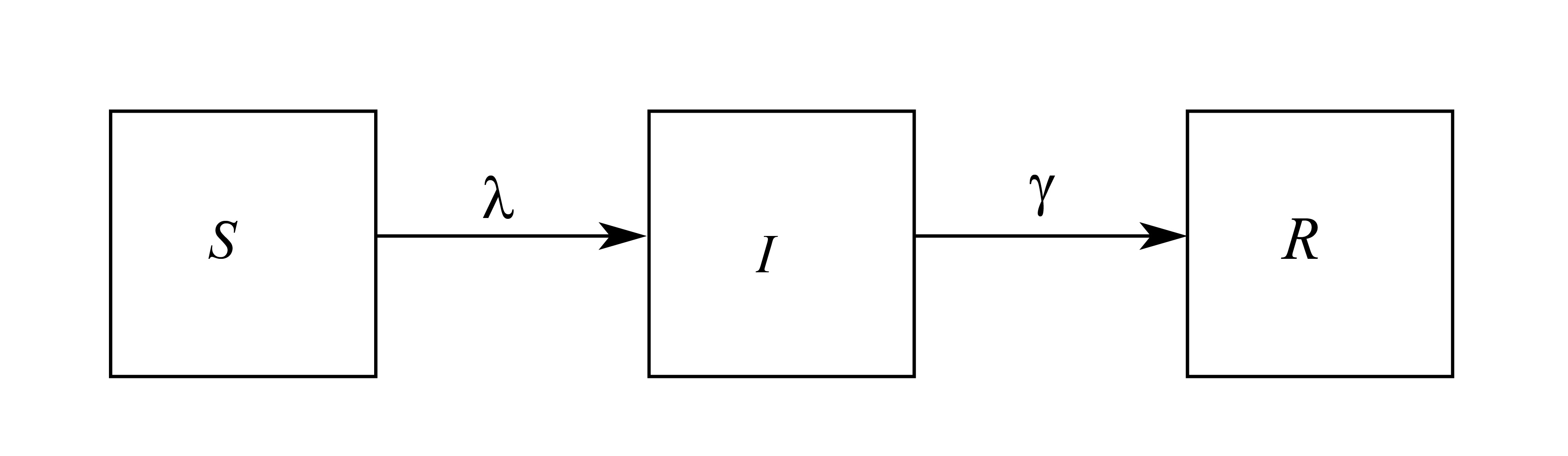
The rate equations for the state variables that describe the model shown in Figure 3 are
\[\begin{array}{l} \frac{dS}{dt} = - \lambda \left(I\right)S \\ \\ \frac{dI}{dt} = \lambda \left(I\right)S- \gamma I \\ \\ \frac{dR}{dt} = \gamma I \\ \end{array} \tag{2}\]
Since the total population N is constant we have the following relationship between S, I, and R.
\[N=S+I+R \tag{3}\]
Therefore, the dynamics of the system are really determined by two rate equations rather than three. The function \(\lambda \left(I\right)\) is called the force of infection and gives the per capita rate at which susceptible individuals acquire infection. Different versions of the SIR model can be defined by choosing different forms for \(\lambda \left(I\right)\). A typical choice is given by
\[\lambda \left(I\right) = \beta \frac{I}{N} \tag{4}\]
\(\beta\) is called the transmission rate.
We can convert the state variables to dimensionless form by dividing by the total population.
\[s = \frac{S}{N}\text{ , }i = \frac{I}{N}\text{ , }r = \frac{R}{N} \tag{5}\]
With these definitions for s, i, and r the rate equations become
\[\begin{array}{left} \frac{ds}{dt} = - \beta si \\ \frac{di}{dt} = \beta si- \gamma i \\ \frac{dr}{dt} = \gamma i \\ \end{array} \tag{6}\]
and the conservation law Equation 3 becomes
\[1=s+i+r \tag{7}\]
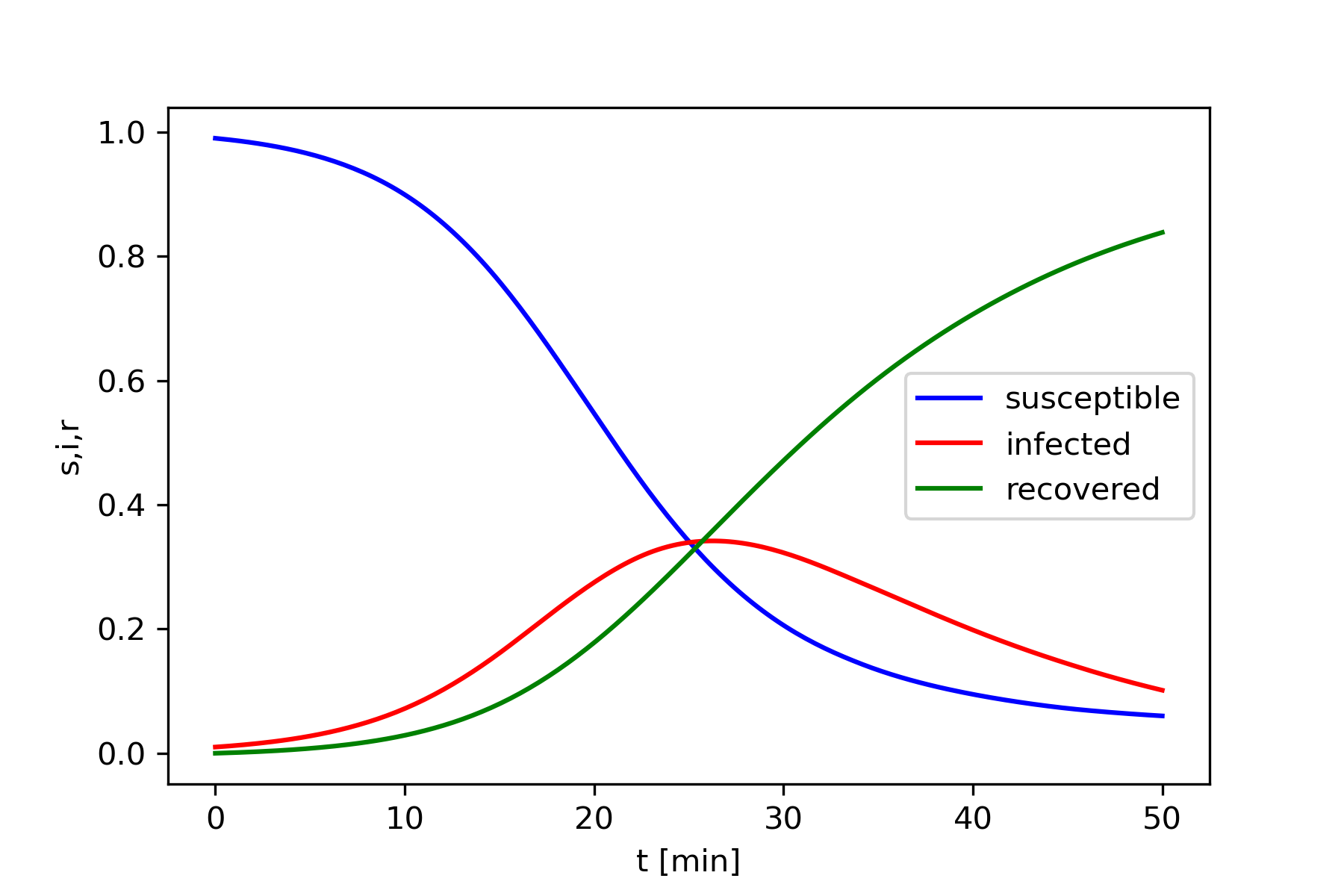
Figure 4 shows an example of the results of this model. This model shows an infection that always dies out eventually with all infected people eventually recovering.
Physics
Bungee Jumping
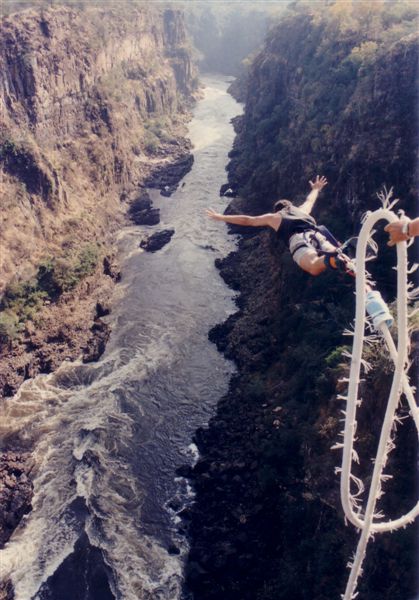
Bungee jumping involves attaching a long bungee cord, a type of elastic cord, to a person and then having the person step off a bridge and plunge downwards, and then be pulled back up by the cord, shown in Figure 5.
|
|
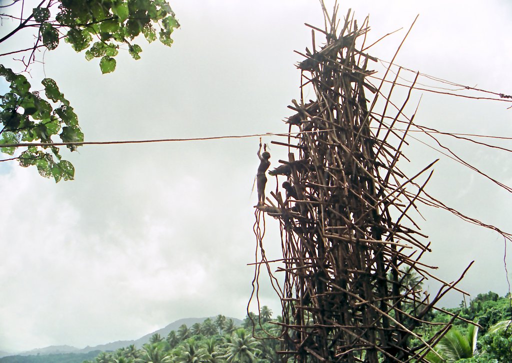
In the modern world it is a popular form of extreme activity, but there are examples of similar activities in history including the land diving ritual performed by men living on Pentecost Island, Vanuatu, shown in Figure 6.
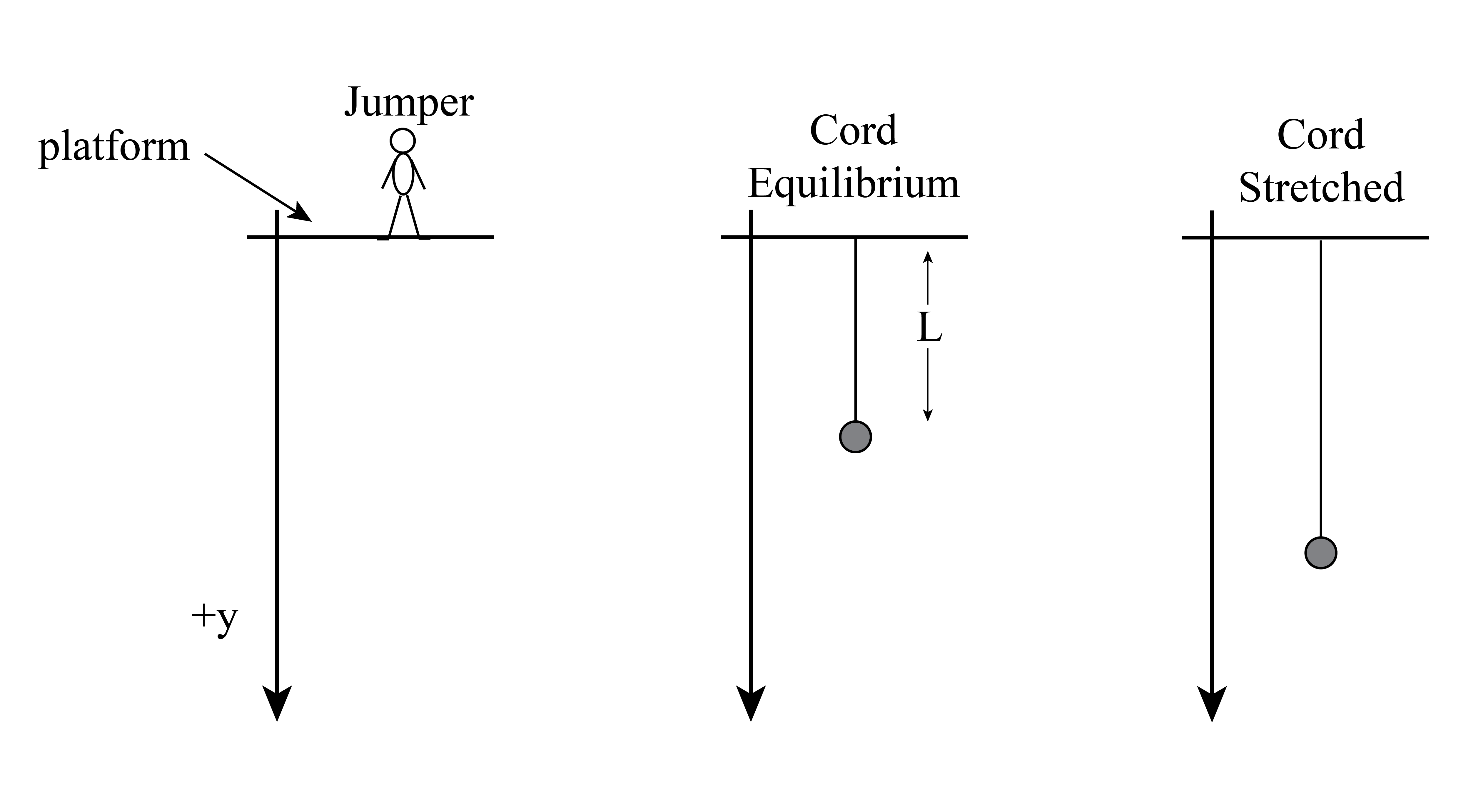
We will develop a basic mathematical model for the trajectory of a jumper using Newton’s Second Law (Menz, 1993). The coordinate system that will be used to describe the jumper’s position is shown in Figure 7. The origin of the y-axis is at the platform where the jumper steps off, and we take the +y direction to be down. The unstretched length of the cord is L. The mass of the jumper is m. We assume the bungee cord is massless.
The y-component of Newton’s Second Law is
\[\begin{array}{l} \sum_iF_{iy} = m\ddot{y} \\ \\ mg- B\left(t\right)H\left(y- L\right)- D\left(t\right) = m\ddot{y} \\ \end{array} \tag{8}\]
which gives
\[\ddot{y} = g- \frac{1}{m}B\left(t\right)H\left(y- L\right)- \frac{1}{m}D\left(t\right) \tag{9}\]
Note that the bungee force is nonzero only when y>L. This fact can be implemented by using the Heaviside function
\[H\left(y\right) = \left\{\begin{array}{cc} 1\text{ , }y \geq 0 \\ 0\text{ , }y < 0 \\ \end{array}\right. \tag{10}\]
The following model for the air drag force will be used.
\[D_y\left(v_y\right) = - \frac{1}{2}\rho C_DA\left(v_y^2\right)sign\left(v_y\right) \tag{11}\]
where
\[\begin{array}{l} \rho = \text{density of air} \\ C_D = \text{dimensionless drag coefficient for the object} \\ A = \text{cross-sectional area of the object} \\ sign\left(v_y\right) = \left\{\begin{array}{cc} + 1\text{ , }v_y > 0 \\ - 1\text{ , }v_y < 0 \\ \end{array}\right. \\ \end{array}\]
We need a model for the bungee force B. The simplest bungee force model is to assume that it acts as an ideal spring
\[B = k_1\left(y- L\right) \tag{12}\]
A more realistic bungee force is suggested by Figure 8

where x is the amount of cord stretch from equilibrium. The equation describing the force implied by this figure is
\[B = \left\{\begin{array}{cc} K_1x\text{ , }0 \leq x \leq X_1 \\ K_2x + \left(K_1- K_2\right)X_1\text{ , }X_1 < x \leq X_2 \\ K_2X_2 + \left(K_1- K_2\right)X_1\text{ , }X_2 < x \\ \end{array}\right. \tag{13}\]
Model Rocket Trajectory
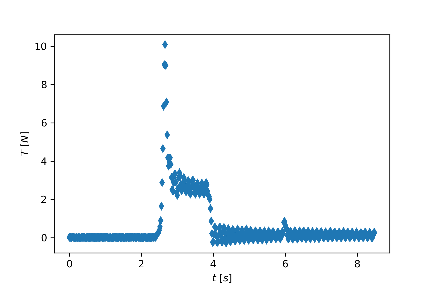
Model rocketry is a popular hobby for many adults and children. The rockets are constructed from cardboard, plastic, and balsa wood and are powered by commercially available solid propellant engines that can generate a thrust force of a few Newtons over one to three seconds (Estes Rockets, 2021). Figure 9 shows an example of the thrust data for a particular engine. The second small thrust peak corresponds to the parachute ejection shot. It can be ignored in the trajectory analysis that follows.
The trajectory of the model rocket can be predicted from the thrust data by performing a Newton’s Second Law analysis. The resulting equations of motion will be most easily studied using a numerical integration procedure, as discussed in previous chapters. The Newton’s 2nd Law analysis begins with a free body diagram. The physical forces acting on the rocket include gravity, \(\overrightarrow{\mathbf F}_g\), the rocket thrust, \(\overrightarrow{\mathbf T}\), and the air drag, \(\overrightarrow{\mathbf D}\). Figure 10 shows the free body diagram and the definition of the +y direction that will be assumed in the analysis.
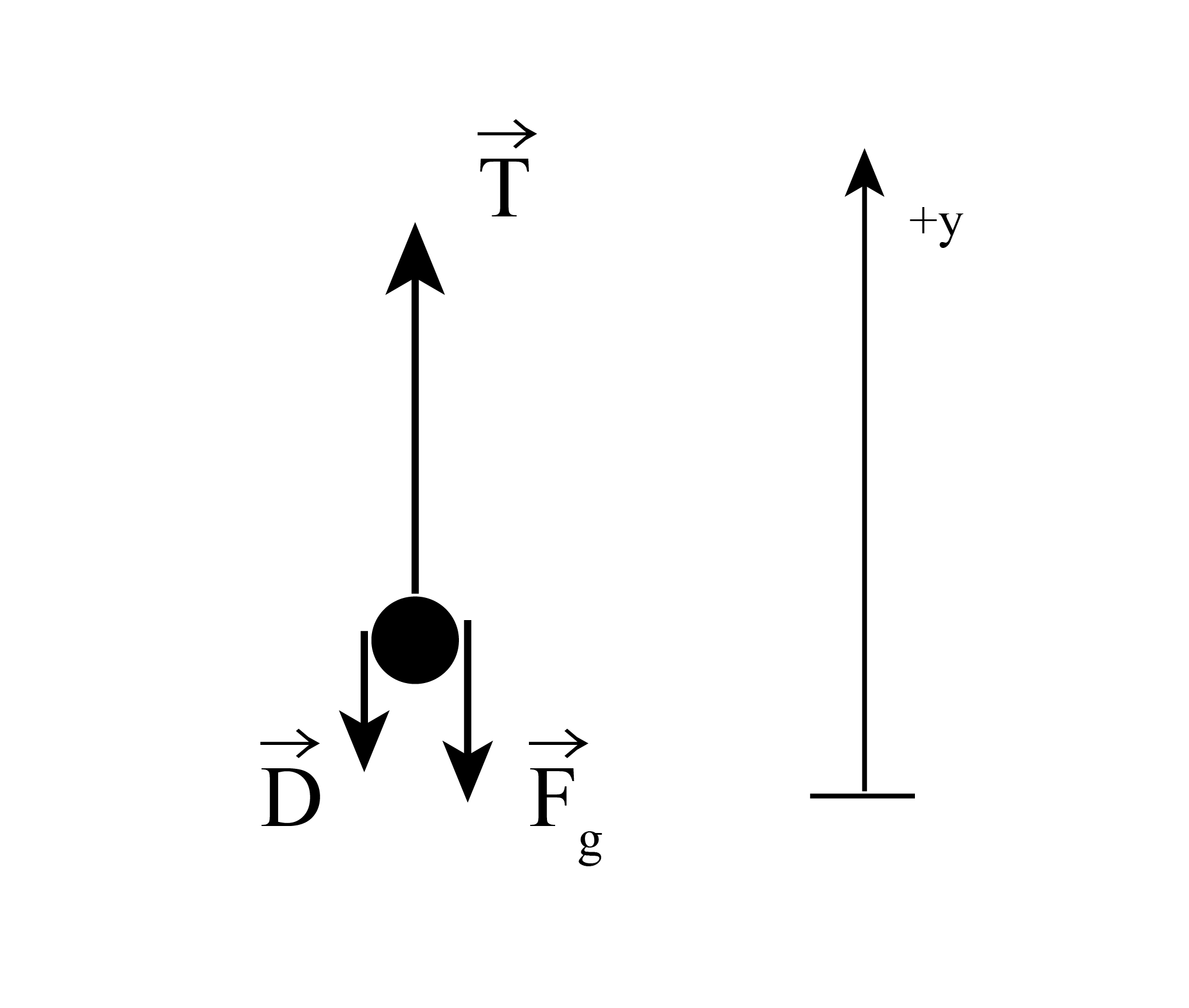
We introduce the following function definitions
\[\begin{array}{l} m\left(t\right) = \text{mass of the rocket and engine as a function of time t} \\ D\left(t\right) = \text{magnitude of the drag force as a function of time} \\ T\left(t\right) = \text{magnitude of the thrust force as a function of time} \\ \end{array}\]
Newton’s Second Law expressed in terms of momentum is
\[\overrightarrow{\text{F}}_{\text{net}} = \frac{d\overrightarrow{\text{p}}}{dt}\text{,}\overrightarrow{\mathbf p} = m\left(t\right)\overrightarrow{\mathbf v} \tag{14}\]
We will assume that the rocket travels only in the vertical direction, so only the y-component of the forces and Newton’s Second Law will be needed.
\[F_{gy} = - m\left(t\right)g \tag{15}\]
The model for the air drag force is given by Equation 11. We also need a model for the thrust function based on the available thrust data. This will be developed below.
Newton’s Second Law, Equation , can now be written as
\[T\left(t\right) + D_y\left(v_y\right)- m\left(t\right)g = \frac{dm}{dt}v_y\left(t\right) + m\left(t\right)a_y\left(t\right) \tag{16}\]
where
\[a_y\left(t\right) = \text{y-component of acceleration at time t}\]
We will assume that the mass of the rocket will not change as the engine burns since the fuel mass is a very small percentage of the total mass. This assumption gives
\[\frac{dm}{dt} = 0 \tag{17}\]
which allows us to write Equation 16 as
\[a_y\left(t\right) = \frac{1}{m}\left[T\left(t\right) + D_y\left(v_y\right)- mg\right] \tag{18}\]
Next, we will develop a mathematical model for the rocket thrust. Figure 9 suggests that a possible mathematical model for the thrust is given by Figure 11.
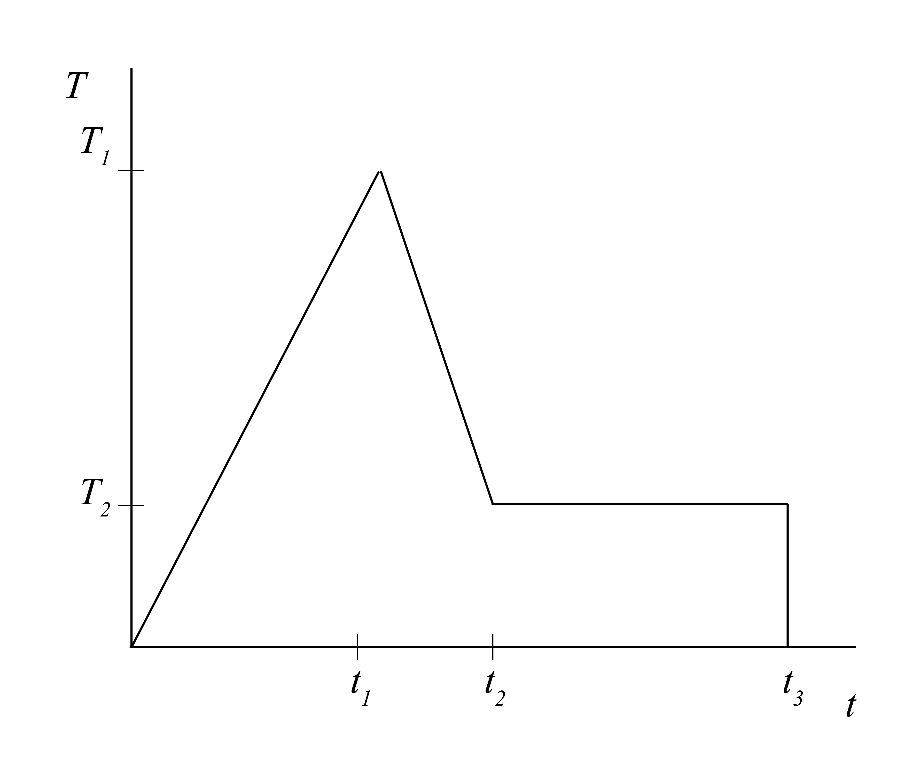
Using analytical geometry, we can find the equation representing Figure 11 to be
\[T\left(t\right) = \left\{\begin{array}{cc} s_1t\text{ , }0 \leq t \leq t_1 \\ s_2t + b\text{ , t}_1 < t \leq t_2 \\ T_2\text{ , }t_2 < t \leq t_3 \\ 0\text{ , t>t}_3 \\ \end{array}\right. \tag{19}\]
where
\[s_1 = \frac{T_1}{t_1}\text{ , }s_2 = \frac{\left(T_2- T_1\right)}{\left(t_2- t_1\right)}\text{ , }b = \left(T_1- s_2t_1\right)\]
Additional background information about model rocket trajectories can be found in Keeports (1990).
Projects
HIV Infection of an Individual
Fit the data in the file HIVData.txt to the HIV model defined by Equation 1 using the least squares method to find the best fit model parameters. Explore how making variations in model parameters affects the time behavior of the infection.
Explore the effect of antiretroviral therapy by modifying the rate equation for V as suggested by Perelson & Ribeiro (2013). First explore how the theoretical predictions for the original model of Equation 1 compare with theoretical predictions of the modified model. Next, locate data on viral concentration after antiretroviral therapy and compare the viral clearance rate, dV, with therapy and without therapy.
Epidemiology of the COVID-19 Infection
Use the data file owid-covid-data.xlsx from the Our World in Data website (Mathieu et al., 2020) to obtain COVID infection data for the US. Fit the US data for the early stage of the epidemic to the model of Equation 6. Is there any time period for which the basic SIR model provides an adequate description? Calculate the basic reproductive rate for the infected population (see Blackwood & Childs (2018) for discussion of the reproductive rate).
Add birth and death terms to the rate equations. Implement a numerical solution to the revised model. Explore the effect of changing birth and death rates on the time behavior of the model. What is the effect of birth and death on the basic reproduction rate?
Bungee Jumping
Implement a numerical solution to the model of Equation 9. Investigate bungee jumping sites to determine typical drop lengths for participants. If possible, determine typical times for a jumper to come to rest. Use this data to determine best fit model parameter values. Explore the behavior of velocity and acceleration over the time of the jump. Use the model to explore possible health effects of bungee jumping.
Implement a numerical solution to the model of Equation 9. Use the model to assist in designing a bungee jump site. You will need to decide about the range of jumper masses your site will accommodate, the maximum jump height, and the required bungee cords that will serve people of different mass. Research safety and health concerns and verify that your design meets all required safety criteria.
Model Rocket Trajectory
Use the thrust data given for the Estes A8-3, B4-2, and B6-2 engines to estimate the parameters for the thrust model given by Equation 18. The thrust data is contained in the files A8-3_ThrustData.txt, B4-2_ThrustData.txt, and B6-2_ThrustData.txt. Create a Python thrust force function for each of the engines. Choose a model rocket from the Estes catalog. Note the rocket’s mass, cross-sectional area, and suggested maximum height. Implement a numerical solution of the trajectory model given by Equation 18 for each of the engines. Compare the theoretical maximum height with the height suggested by Estes.
Develop a mathematical model for a two-dimensional rocket trajectory. This will require analyzing motion in both the vertical and horizontal directions. Explore how the launch angle affects the maximum height and range of the rocket for each of the engines.
References
Adiga, A., Dubhashi, D., Lewis, B., Marathe, M., Venkatramanan, S., & Vullikanti, A. (2020). Mathematical Models for COVID-19 Pandemic: A Comparative Analysis. Journal of the Indian Institute of Science, 100(4), 793–807. https://doi.org/10.1007/s41745-020-00200-6
Blackwood, J., & Childs, L. (2018). An introduction to compartmental modeling for the budding infectious disease modeler. Letters in Biomathematics, 5(1), Article 1. https://doi.org/10.30707/LiB5.1Blackwood
Estes Rockets. (2021). Estes Industries. https://estesrockets.com/
Keeports, D. (1990). Numerical calculation of model rocket trajectories. The Physics Teacher, 28(5), 274–280. https://doi.org/10.1119/1.2343024
Levy, J. A. (1993). Pathogenesis of human immunodeficiency virus infection. Microbiological Reviews, 57(1), 183–289. https://doi.org/10.1128/mr.57.1.183-289.1993
Mathieu, E., Ritchie, H., Rodés-Guirao, L., Appel, C., Giattino, C., Hasell, J., Macdonald, B., Dattani, S., Beltekian, D., Ortiz-Ospina, E., & Roser, M. (2020). Coronavirus Pandemic (COVID-19). Our World in Data. https://ourworldindata.org/coronavirus-source-data
Menz, P. G. (1993). The physics of bungee jumping. The Physics Teacher, 31(8), 483–487. https://doi.org/10.1119/1.2343852
Perelson, A. S., & Ribeiro, R. M. (2013). Modeling the within-host dynamics of HIV infection. BMC Biology, 11, 96. https://doi.org/10.1186/1741-7007-11-96
Ribeiro, R. M., & Perelson, A. S. (2004). The Analysis of HIV Dynamics Using Mathematical Models. In AIDS and Other Manifestations of HIV Infection (4th ed.). Elsevier.
Spy007au. (1996). Bungee jumping off the Zambezi Bridge, Victoria Falls, Africa. Own work by the original uploader. https://commons.wikimedia.org/wiki/File:Bill%27s_Bungy_Jump.jpg
Stein, P. (2010). The Tower. https://commons.wikimedia.org/w/index.php?curid=10438782
WHO Coronavirus (COVID-19) Dashboard. (2020). WHO Coronavirus (COVID-19) Dashboard. https://covid19.who.int
Wikipedia Contributors. (2022). HIV. In Wikipedia. https://en.wikipedia.org/w/index.php?title=HIV&oldid=1119384291