Dynamical Systems Modeling II
Chapter 7 introduced the concept of a dynamical system, a type of deterministic mathematical model with behavior determined by a first-order differential equation, the rate equation for the state variable. This chapter will expand the type of model that we can study to include more than one state variable. One consequence of this generalization is that we will develop the capability to solve problems based on a Newton’s second law analysis of a system. This will open up significant areas of physics and engineering to us.
Motivating Problem: The Zombie Apocalypse
Zombies are a fixture of modern popular culture. Wikipedia currently lists 588 movies with a zombie theme (Wikipedia Contributors, 2022). If we add in all of the television series, comics, novels, short stories, and electronic games, the list of zombie-themed entertainment titles would undoubtedly be in the thousands. Even the Center for Disease Control offers a pamphlet on preparing for a zombie pandemic (Centers for Disease Control and Prevention (U.S.) & Office of Public Health Preparedness and Response, 2011).
The first Hollywood box-office hit with a zombie theme was White Zombie, released in 1932 and starring Bela Lugosi, of Dracula fame, as Voodou master “Murder” Legendre, who kills and resurrects people as zombies using a potion (Kay & Brugués, 2012). The zombies in this film are mindless beasts controlled by their maker, not the brain-eating, decayed flesh monstrosities of more modern productions.
The 1968 film Night of the Living Dead defined critical elements of the modern zombie genre: normal humans become infected from the bite of a zombie, an infected person dies and becomes reanimated with an appetite for human flesh, and a zombie can be killed with a shot to the base of the skull or by fire. Night of the Living Dead did not use the term zombie for the reanimated, flesh-eating wanderers. These creatures were called ghouls in the movie.
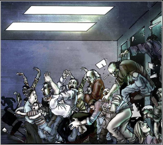
The modern zombie story views the condition as an infectious disease spread through close contact with uninfected people. Typically, the infection is incredibly successful at spreading through the human population, leaving the world with a huge number of roaming, flesh-eating creatures in the midst of a dwindling number of humans. fig-Figure8ZombiePandemic shows one depiction of such a pandemic, as visualized by an artist at the U.S. Centers for Disease Control (Centers for Disease Control and Prevention (U.S.) & Office of Public Health Preparedness and Response, 2011). Our modeling problem is to understand the conditions for which the zombie infection can spread so as to essentially wipe out the human population. A related question is, what are the conditions that will allow humans to make a comeback?
Compartmental Models
Compartmental models are a class of mathematical model for which the system under investigation is assumed to be composed of populations that can exist in one or more states or compartments. Each compartment can be described by one state variable and flows can occur between the compartments. In addition to flows between compartments, other processes that affect the population in a compartment can be included, such as birth and death events.
Compartmental models have become useful in many areas of science and engineering including chemical engineering, ecology, environmental engineering, epidemiology, pharmacokinetics, and physiology. To introduce the concept, we will focus on developing a compartmental model of a chemostat, a type of bioreactor used in microbiology research and in bioengineering applications.
A chemostat provides a continuous supply of microorganisms using constant and reproducible growth conditions. This allows the microorganisms to be used in research or industrial applications under predictable and controllable conditions. Figure 2 shows the conceptual physical structure of a chemostat.
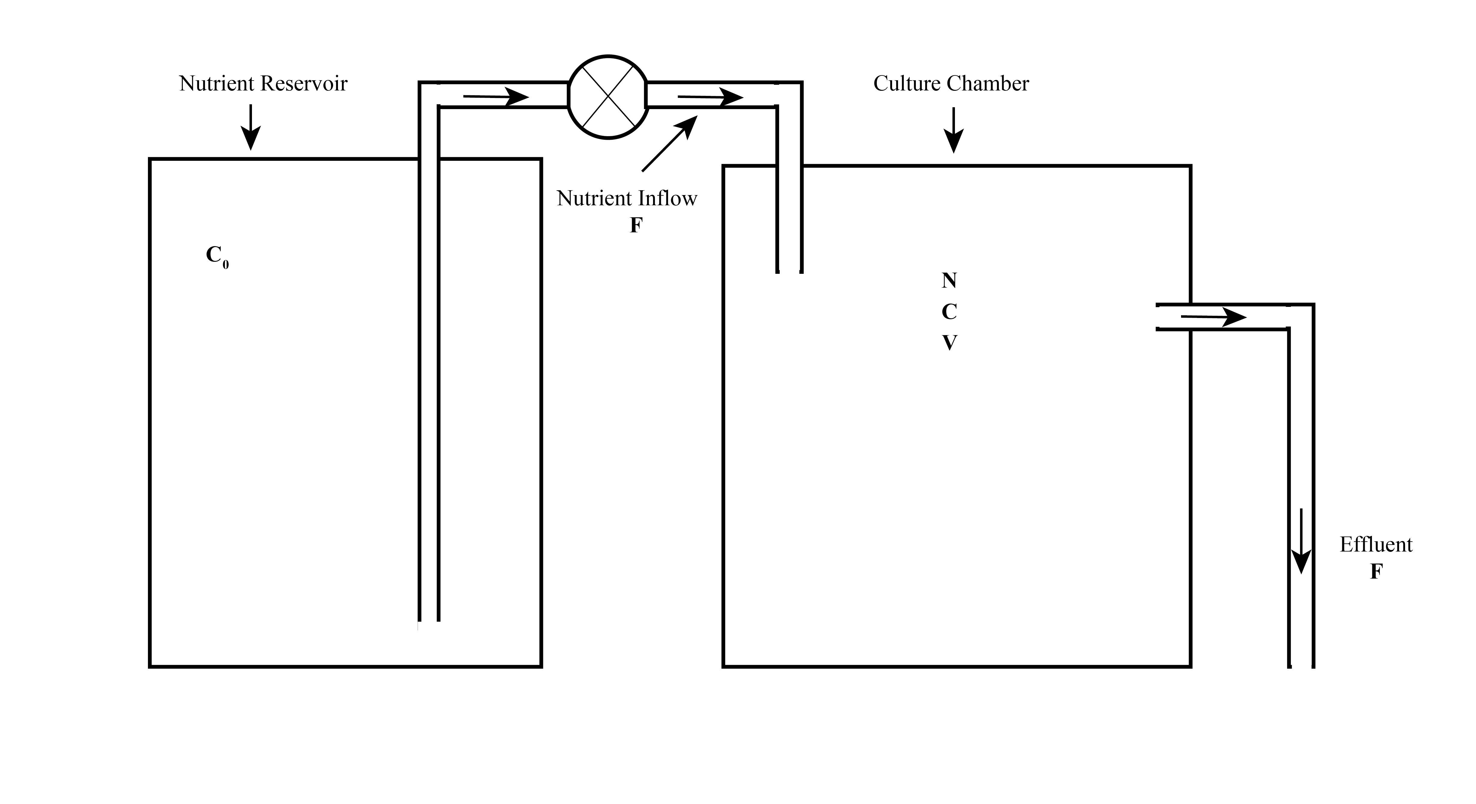
We can start constructing a mathematical model of this device defining important variables or parameters that describe the system.
| Variable | Symbol | Units | Units Example | ||
|---|---|---|---|---|---|
|
N | cells/volume | cells/ml | ||
|
C | mass/volume | g/ml | ||
|
C0 | mass/volume | g/ml | ||
| Volume of the culture chamber | V | volume | ml | ||
| Nutrient inflow and effluent outflow rate | F | volume/time | ml/s |
We will make some assumptions about our system to keep our model relatively simple.
The nutrient reservoir will always supply nutrient at the fixed concentration C0.
The nutrient inflow rate will always equal the outgoing effluent rate, F. This will keep the volume of the culture chamber constant.
The culture chamber is well mixed, so the bacteria and nutrient concentrations are constant throughout.
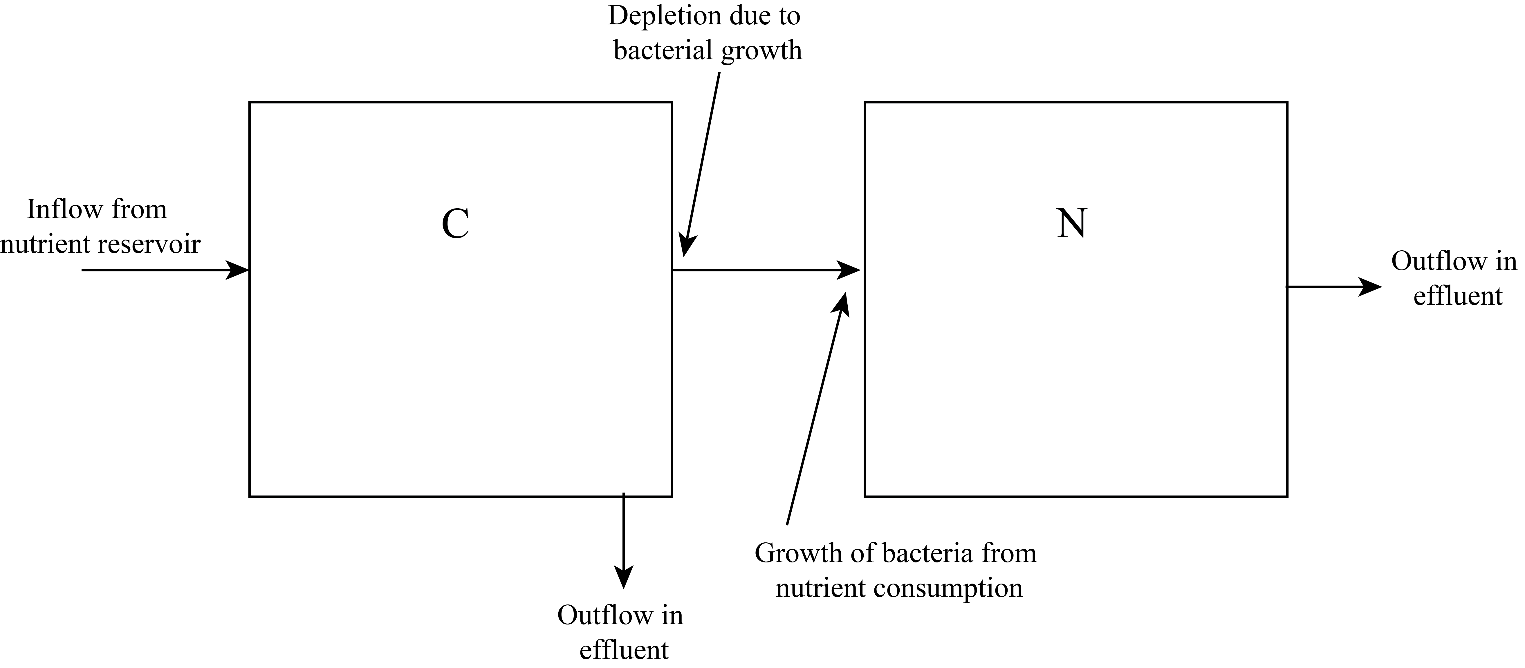
With these assumptions we can focus our attention on the culture chamber containing both the bacteria and the nutrient. Our system can be modeled conceptually by two compartments: a bacteria compartment and a nutrient compartment. Our conceptual compartmental model of the system is represented in Figure 3.
To define the dynamical system model we must specify rate equations for the two state variables, N and C. This will require some additional model parameters, defined in Table 2.
| Parameter | Symbol | Units |
|---|---|---|
| the yield constant | Y | (cells/volume)/(mass/volume) |
| specific growth rate | K | 1/time |
| maximum specific growth rate | \(K_{max}\) | 1/time |
| saturation constant | \(K_s\) | mass/volume |
The rate equation for a state variable must contain terms corresponding to each arrow going into or out from the associated compartment in Figure 8.3. Following Leah Edelstein-Keshet, we will hypothesize the following rate equations (Edelstein-Keshet, 2005).
\[\frac{dN}{dt} = K\left(C\right)N- \frac{FN}{V} \tag{1}\]
\[\frac{dC}{dt} = - \frac{K\left(C\right)N}{Y}- \frac{FC}{V} + \frac{FC_0}{V} \tag{2}\]
The specific growth rate, K, is assumed to be a function of the nutrient concentration, C. The yield constant, Y, maximum specific growth rate, Kmax, and the saturation constant, Ks, will depend on the species of bacteria being modeled.
We must also hypothesize a model for the specific growth rate. A realistic model should show the growth rate reaching a maximum for large values of the nutrient concentration. A commonly used model is described by Michaelis-Menten kinetics equation (Edelstein-Keshet, 2005):
\[K\left(C\right) = \frac{K_{\max}C}{K_s + C} \tag{3}\]
With this choice for the growth kinetics model, the rate equations become
\[\frac{dN}{dt} = \left(\frac{K_{\max}C}{K_s + C}\right)N- \frac{FN}{V} \tag{4}\]
\[\frac{dC}{dt} = - \left(\frac{K_{\max}C}{K_s + C}\right)\frac{N}{Y}- \frac{FC}{V} + \frac{FC_0}{V} \tag{5}\]
This model has six parameters: Kmax, Ks, Y, V, F, C0. Exploring the behavior of the model can be complicated with so many parameters. Another complication that arises in performing numerical solutions of the model is that there can be a large range of numbers involved. Both of these complications can be mitigated to some extent by rewriting the equations in a dimensionless form. This can be done by writing the original variables N, C, and t as the product of a dimensionless variable and a dimensional number (Edelstein-Keshet, 2005).
\[\begin{array}{l} N = N^* \times \widehat{N} \\ C = C^* \times \widehat{C} \\ t = t^* \times \widehat{t} \\ \end{array} \tag{6}\]
In these definitions, \(N^*\), \(C^*\), and \(t^*\) are the new dimensionless variables and \(\widehat{N},\widehat{C},\text{ and }\widehat{t}\) are constants that contain dimensions. Our goal is to choose the values of these dimension-carrying constants in a way that reduces the number of model parameters in Equation 4 and Equation 5. Substituting the definitions from Equation 6 into Equation 4 and Equation 5 yields Equation 7 and Equation 8.
\[\frac{dN^*}{dt^*} = \widehat{t}K_{\max}\left(\frac{C^*}{K_s/ \widehat{C} + C^*}\right)N^*- \widehat{t}\frac{FN^*}{V} \tag{7}\]
\[\frac{dC^*}{dt^*} = - \left(\frac{\widehat{t}K_{\max}\widehat{N}}{Y\widehat{C}}\right)\left(\frac{C^*}{K_s/ \widehat{C} + C^*}\right)N^*- \widehat{t}\frac{FC^*}{V} + \widehat{t}\frac{FC_0}{V\widehat{C}} \tag{8}\]
By choosing the dimensional constants \(\widehat{N},\widehat{C},\text{ and }\widehat{t}\) appropriately, the number of independent model parameters can be reduced. The following choice yields two model parameters.
\[\widehat{t} = \frac{V}{F}\text{ , }\widehat{C} = K_s\text{ , }\widehat{N} = \frac{YK_s}{\widehat{t}K_{\max}} \tag{9}\]
To facilitate performing a numerical solution of these equations to give N* and C* as functions of time, we will change the notation to the generic dynamical systems model notation.
\[\begin{array}{l} N^*\rightarrow y_0 \\ C^*\rightarrow y_1 \\ \end{array} \tag{10}\]
Making the substitutions defined in Equation 9 and the notation change defined by Equation 10 gives the final form of our dynamical systems model.
\[\frac{dy_0}{dt} = a_1\left(\frac{y_1}{1 + y_1}\right)y_0- y_0 \tag{11}\]
\[\frac{dy_1}{dt} = - \left(\frac{y_1}{1 + y_1}\right)y_0- y_1 + a_2 \tag{12}\]
where
\[\begin{array}{l} a_1 = \widehat{t}K_{\max} = \frac{VK_{\max}}{F} \\ \\ a_2 = \frac{\widehat{t}FC_0}{V\widehat{C}} = \frac{C_0}{K_s} \\ \end{array} \tag{13}\]
The model parameters a1 and a2 are dimensionless.
The dynamical systems model defined by Equations (8.11) and (8.12) can be solved numerically by using the code template from Figure 7.7. Figure 4 shows the Figure 7.7 code adapted for the chemostat problem. Figure 5 shows the result of running the code. For these model parameter values, it takes about 40 dimensionless time units to achieve a stable steady-state production of bacteria.
"""
Program: Chemostat Model
Author: C.D. Wentworth
Version: 8.22.2022.1
Summary:
    This program implements a dynamical systems model of a
    chemostat that uses one growth-limiting nutrient and
    produces one species of bacteria. The model is expressed in
    a dimensionless form.
Version History:
    8.22.2022.1: base

"""
import scipy.integrate as si
import numpy as np
import matplotlib.pylab as plt

# Create a function that defines the rhs of the differential equation system

def f(t, y, a1, a2):
    #   y = a list that contains the system state
    #   t = the time for which the right-hand-side of the system equations
    #       is to be calculated.
    #   a1 = a parameter needed for the model
    #   a2 = a paramteter needed for the model

    #   Unpack the state of the system
    y0 = y[0]  # N*
    y1 = y[1]  # C*

    #   Calculate the rates of change (the derivatives)
    dy0dt = a1*(y1/(1.0 + y1))*y0 - y0
    dy1dt = -(y1/(1.0 + y1))*y0 - y1 + a2

    return [dy0dt, dy1dt]

# Main Program

# Define the initial conditions
yi = [0.01, 5.0]

# Define the time grid
ti = 0.0
tf = 15.0
t = np.linspace(ti, tf, 200)

# Define the parameter tuple
#a1 = 2.6  #
a1 = 2.67
a2 = 5.0  #
p = (a1, a2)

# Solve the DE
sol = si.solve_ivp(f, (ti, tf), yi, t_eval=t, args=p)
N = sol.y[0]
C = sol.y[1]

# Plot the solution
plt.plot(t, N, color='green', label='N*')
plt.plot(t, C, color='red', label='C*')
plt.xlabel('t*')
plt.ylabel('N* , C*')
plt.legend()
plt.savefig('chemostat.png')
plt.show()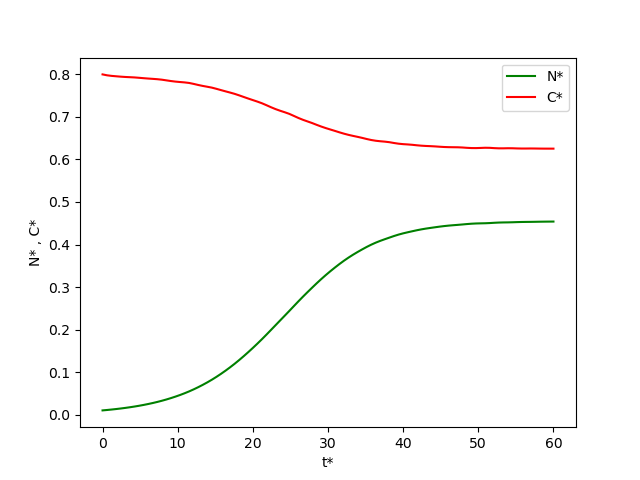
Numerical Solution of 2nd-Order Differential Equations
Many scientific and engineering systems can be modeled with second-order differential equations. One reason this is the case is that Newton’s second law is really a second-order differential equation.
\[F_{net} = ma_x = m\frac{d^2x}{dt^2} \tag{14}\]
We can solve such an equation numerically without being expert mathematicians by using our ability to solve a first-order equation numerically, as done in our dynamical systems models. We can make use of the dynamical systems approach to numerical solution by using a nice trick to turn a second-order differential equation into two first-order differential equations.
The key will be to define a new set of variables that produce a new model that is simply related to the old second-order differential equation model. We will learn how to define the new variables by considering a specific example. Equation 15 defines a second-order differential equation.
\[\frac{d^2y\left(t\right)}{dt^2} + q\left(t\right)\frac{dy\left(t\right)}{dt} = r\left(t\right) \tag{15}\]
where we assume that the functions \(q\left(t\right)\) and \(r\left(t\right)\) are known. Define a new set of variables \(y_0\left(t\right)\) and \(y_1\left(t\right)\) as follows
\[\begin{array}{left} y_0 = y \\ y_1 = \frac{dy}{dt} \\ \end{array} \tag{16}\]
The rate of change of \(y_1\left(t\right)\) can be obtained from the original second-order differential equation:
\[\frac{d^2y\left(t\right)}{dt^2} = r\left(t\right)- q\left(t\right)\frac{dy\left(t\right)}{dt}\Rightarrow \frac{dy_1\left(t\right)}{dt} = r\left(t\right)- q\left(t\right)y_1\left(t\right) \tag{17}\]
This is due to the second derivative of y being equal to the first derivative of y1. So, Equation 15 can be replaced by the following set of first-order differential equations:
\[\begin{array}{left} \frac{dy_0\left(t\right)}{dt} = y_1\left(t\right) \\ \frac{dy_1\left(t\right)}{dt} = r- qy_1\left(t\right) \\ \end{array} \tag{18}\]
If we solve this system numerically, then we will have also solved Equation 15 for y(t), since that is just the new variable y0.
Newton’s 2nd Law Problems
Let’s look at performing a numerical solution to a specific problem: a mass attached to a spring. This is a good testing problem since it can be solved exactly without performing the numerical solution. This will allow us to verify our numerical approach.
Figure 6 shows the scenario: a block of mass 0.15 [kg] is attached to a spring with spring constant of 20 [N/m]. The mass is stretched a distance x0 = 0.10 [m] and released from rest. The state variable x will be the position of the mass measured from the spring’s unstretched position.
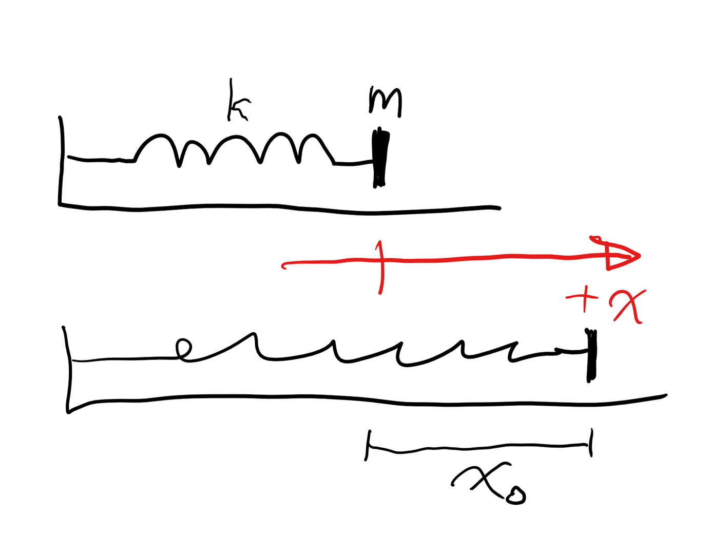
We can create a model of the object’s motion by using Newton’s second law and Hooke’s law for the spring force, which is the only force in the x direction.
\[F_{net} = m\frac{d^2x}{dt^2} \tag{19}\]
\[F_s = - kx \tag{20}\]
Combining these equations leads to our model for x:
\[\frac{d^2x\left(t\right)}{dt^2} = - \frac{k}{m}x\left(t\right) \tag{21}\]
Now we apply our trick to turn the second-order differential equation into two first-order equations. We define new state variables \(y_0\left(t\right)\) and \(y_1\left(t\right)\):
\[\begin{array}{left} y_0 = x \\ y_1 = \frac{dy_0}{dt} \\ \end{array} \tag{22}\]
The rate equations for our new state variables are
\[\begin{array}{left} \frac{dy_0}{dt} = y_1 \\ \frac{dy_1}{dt} = - \frac{k}{m}y_0 = - \frac{20\left[N/ m\right]}{0.15\left[kg\right]}y_0 \\ \end{array} \tag{23}\]
with the initial conditions
\[y_0\left(0\right) = x_0 = 0.10\left[m\right]\text{ , }y_1\left(0\right) = 0\]
The model is now in a form that can be solved numerically using our Dynamical Systems Template adapted to this model. Figure 7 shows the code that will solve this model numerically. Figure 8 shows the graphical output produced by the code.
"""
Program: Ideal Spring Simulation
Author: C.D. Wentworth
Version: 2.20.2022.1
Summary:
    This program implements a dynamical systems model of the
    one-dimensional ideal spring (Hooke's Law).
Version History:
    2.20.2022.1: base


"""

import scipy.integrate as si
import numpy as np
import matplotlib.pylab as plt

# Create a function that defines the rhs of the differential equation system

def f(t, y, m, k):
    #   y = a list that contains the system state
    #   t = the time for which the right-hand-side of the system equations
    #       is to be calculated.
    #   k = a parameter needed for the model - force constant
    #   m = a paramteter needed for the model - mass

#   Unpack the state of the system
    y0 = y[0]  # x
    y1 = y[1]  # vx

#   Calculate the rates of change (the derivatives)
    dy0dt = y1
    dy1dt = -(k/m)*y0

    return [dy0dt, dy1dt]

# Main Program

# Define the initial conditions
yi = [0.10, 0.0]

# Define the time grid
ti = 0.0
tf = 2.0
t = np.linspace(ti, tf, 100)

# Define the parameter tuple
m = 0.15  # mass in [kg]
k = 20.0  # force constant in [N/m]
p = (m, k)


# Solve the DE
sol = si.solve_ivp(f, (ti, tf), yi, t_eval=t, args=p)
x = sol.y[0]
vx = sol.y[1]


# Plot the solution
plt.plot(t, x, color='green', label='x')
plt.xlabel('t [s]')
plt.ylabel('x [m]')
plt.savefig('idealSpring.png')
plt.show()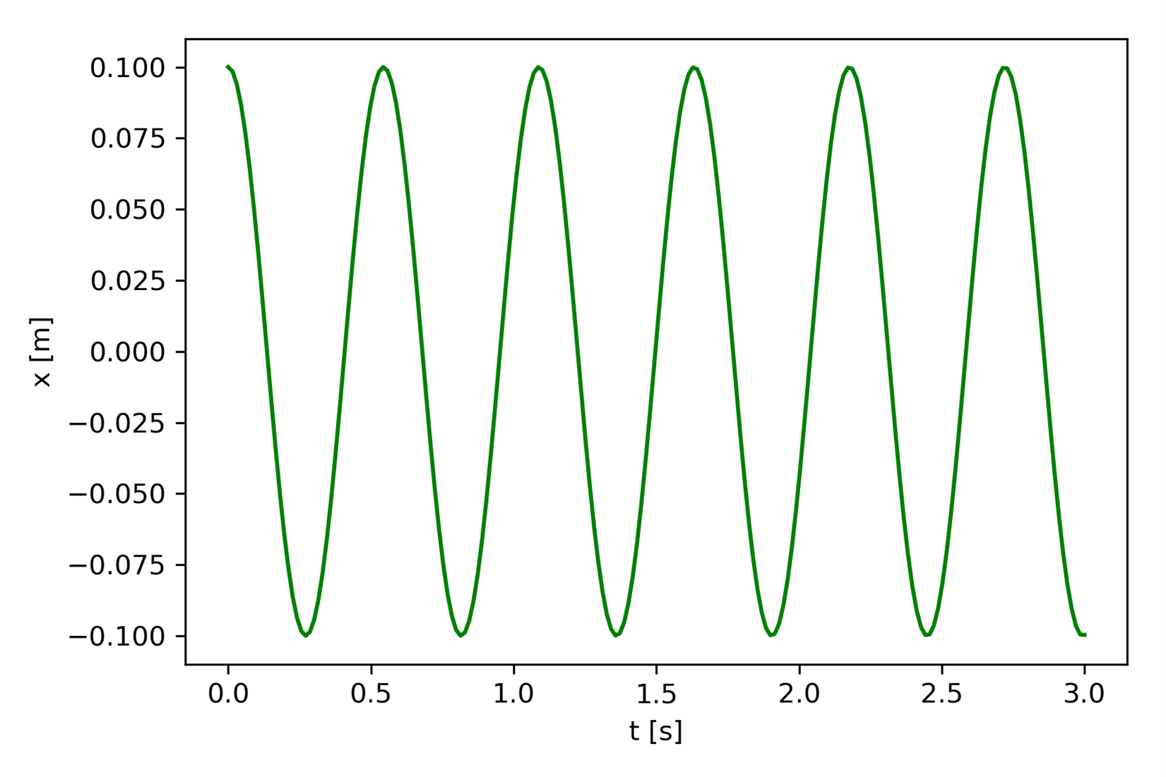
Computational Problem Solving: Modeling the Zombie Apocalypse
We now return to the problem of modeling the Zombie Apocalypse introduced at the beginning of the chapter.
Analysis
The zombie problem we will model is one where it is an infectious disease that requires contact between a susceptible person and an undead individual. We will use a recently published academic study of this type of zombie by infectious disease scientists to help us develop a model (Munz et al., 2009). The population of humans and zombies is assumed to be composed of three compartments:
Susceptibles (S)
Zombie (Z)
Removed (R)
Assumptions we will make include
The susceptible population can die of natural causes.
The susceptible population can increase due to natural growth (birth).
The removed compartment contains humans who have died from natural causes and from fatal zombie encounters.
Members of the removed compartment can resurrect as zombies.
The zombie compartment can increase due to non-fatal susceptible-zombie interactions (infection) or from resurrection from the removed compartment.
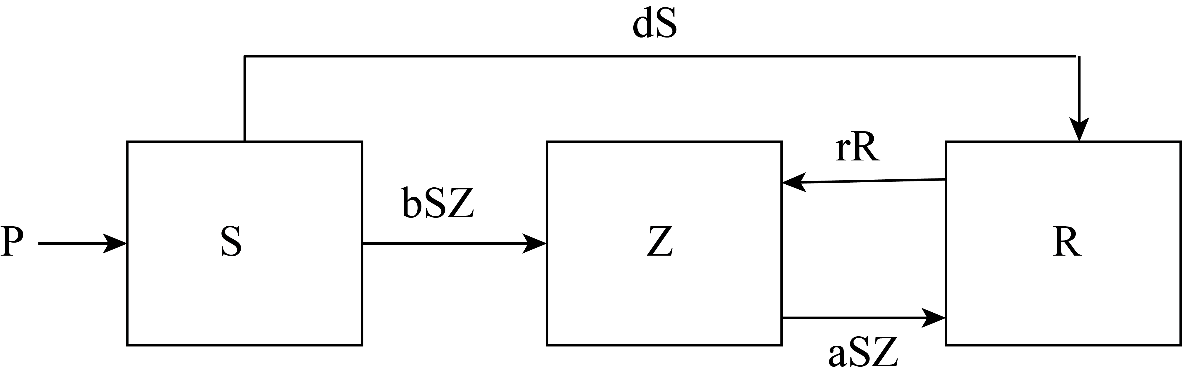
Figure 9 shows the compartmental model hypothesized by Munz, et al. (Munz et al., 2009). Table 3 lists the state variables and parameters used in the model.
| Variable or Model Parameter | Symbol |
|---|---|
| Susceptible Population | S |
| Zombie Population | Z |
| Removed Population | R |
| Constant Birth Rate for Susceptibles | P |
| Natural Death rate for Susceptibles | d |
| Rate at which Susceptible-Zombie encounters produce Zombies | b |
| Rate at which Susceptible-Zombie encounters produce dead Zombies | a |
| Rate at which Removed individuals resurrect as Zombies | r |
Design
Defining the dynamical systems model for our zombie infection requires hypothesizing rate equations for each of the state variables. The compartmental model diagram shown in Figure 9 suggest the following rate equations.
\[\frac{dS}{dt} = P- bSZ- dS \tag{24}\]
\[\frac{dZ}{dt} = bSZ + rR- aSZ \tag{25}\]
\[\frac{dR}{dt} = dS + aSZ- rR \tag{26}\]
We can use the dynamical systems template from Figure 7.7 to perform a numerical solution of this system. The code implementation will be facilitated by making the following notation change.
\[\begin{array}{l} S\rightarrow y_0 \\ Z\rightarrow y_1 \\ R\rightarrow y_2 \\ \end{array} \tag{27}\]
The rate equations Equation 24 - Equation 26 become
\[\frac{dy_0}{dt} = P- by_0y_1- dy_0 \tag{28}\]
\[\frac{dy_1}{dt} = by_0y_1 + ry_2- ay_0y_1 \tag{29}\]
\[\frac{dy_2}{dt} = dy_0 + ay_0y_1- ry_2 \tag{30}\]
Implementation
Performing a numerical solution for the model described by Equation 28 - Equation 30 is straightforward. We must add one more rate calculation in the Python f function and pass the required model parameters. The revised code is in Figure 10 and in the code file SZRModel.py. The units for the compartment populations is arbitrary. The initial conditions must specify a nonzero number for the zombie compartment for there to be any infection activity.
"""
Program: SZR Model
Author: C.D. Wentworth
Version: 8.28.2022.1
Summary:
    This program implements a dynamical systems model of a
    zombie infection based on a three compartment model.
Version History:
    8.28.2022.1: base

"""
import scipy.integrate as si
import numpy as np
import matplotlib.pylab as plt

# Create a function that defines the rhs of the differential equation system

def f(t, y, P, b, d, a, r):
    #   y = a list that contains the system state
    #   t = the time for which the right-hand-side of the system equations
    #       is to be calculated.
    #   a1 = a parameter needed for the model
    #   a2 = a paramteter needed for the model

    #   Unpack the state of the system
    y0 = y[0]  # S
    y1 = y[1]  # Z
    y2 = y[2]  # R

    #   Calculate the rates of change (the derivatives)
    dy0dt = P - b*y0*y1 - d*y0
    dy1dt = b*y0*y1 + r*y2 - a*y0*y1
    dy2dt = d*y0 + a*y0*y1 - r*y2

    return [dy0dt, dy1dt, dy2dt]


# Main Program

# Define the initial conditions
yi = [100, 0.1, 0.0]

# Define the time grid
ti = 0.0
tf = 30.0
t = np.linspace(ti, tf, 100)

# Define the parameter tuple
P = 0.1
b = 9.5e-3
d = 1.e-4
a = 5e-3
r = 1.e-4
p = (P, b, d, a, r)

# Solve the DE
sol = si.solve_ivp(f, (ti, tf), yi, t_eval=t, args=p)
S = sol.y[0]
Z = sol.y[1]
R = sol.y[2]

# Plot the solution
plt.plot(t, S, color='green', label='S')
plt.plot(t, Z, color='red', linewidth=3, label='Z')
plt.plot(t, R, color='blue', linestyle='--', label='R')
plt.xlabel('t')
plt.ylabel('S , Z , R')
plt.legend()
plt.savefig('SZRModel.png')
plt.show()Testing
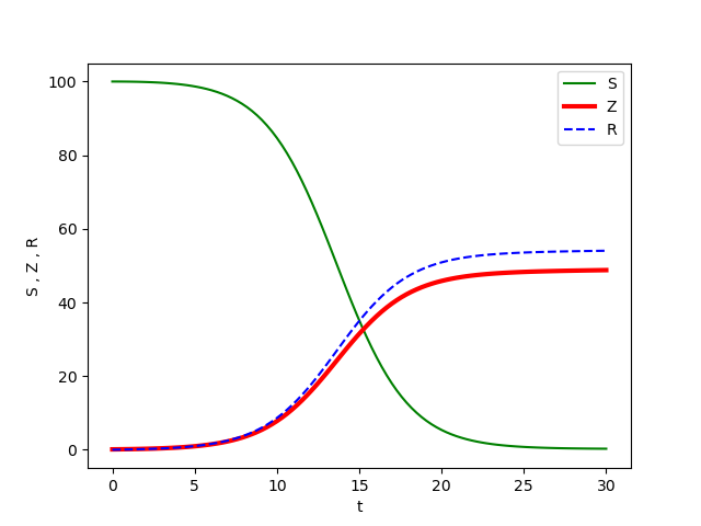
When the code in Figure 10 is executed with the model parameter choices given in lines 49-53 and with the initial conditions in line 41, the result is shown in Figure 11. We see that the susceptible population (uninfected humans) eventually goes to a small number close to zero and the number of zombies and removed become constant. This behavior is consistent with many zombie movies and television shows, which tend to show zombies wiping out most of the human population. This provides some evidence that our model and numerical implementation of its solution are correct.
Exercises
1. True/False: The compartments that are used in a compartmental model must correspond to actual physical containers.
2. True/False: A Newton’s second law problem cannot be solved numerically using the dynamical systems template developed in Chapter 7 since Newton’s second law yields a second-order differential equation rather than just a first-order equation. (Explain your answer.)
3. Replace the following second-order differential equation with two first-order equations.
\[\frac{d^2x}{dt^2} + at^2\frac{dx}{dt} = e^{- bt}\]
4. A chemostat is used to provide a continuous supply of Pseudomonas aeruginosa bacteria for a research project. The following parameters are used for modeling the chemostat (Robinson et al., 1984):
\[\begin{array}{l} K_{\max} = 0.40\left[\text{h}^{\text{-1}}\right] \\ K_s = 2.0 \times 10^{- 3}\left[\frac{mg}{mL}\right] \\ Y = 0.30\left[\frac{\text{mg cell}}{\text{mg Gl}}\right] \\ V = 500.\left[\text{mL}\right] \\ F = 75\left[\frac{\text{mL}}{\text{h}}\right] \\ C_0 = 1.0 \times 10^{- 2}\left[\frac{\text{mg}}{\text{mL}}\right] \\ \end{array}\]
Glucose is used as the nutrient in this reactor. When the chemostat achieves steady-state, the dimensionless state variable values are
\[N* = 11.7\text{ , }C* = 0.599\]
Using the dimensional constants defined by Equation 9, find the actual steady-state values for the cell concentration, in (mg/mL), and the glucose concentration, in (mg/mL), in the chemostat vessel.
Program Modification Problems
1. Consider a large ball dropped from rest from a height. It will experience the force of gravity and an air drag force as it falls. The net force on the ball will be
\[F_{\text{net}} = - mg + kv_y^2\]
You need to develop a model for the ball’s motion as it drops. After developing the equations describing the model, create a Python program that solves for the position of the ball as it drops. Use the following data:
m = 0.220 [kg]
k = 3.7x10⁻²[Ns2/m2]
y(0) = 12 [m]
The program should create a graph of the ball’s position up to the time that it hits the ground. Also, include a calculation of the position as a function of time for the constant acceleration case (no air drag). You can start with the code in Figure 7, which is in the code file idealSpring.py.
2. Consider the chemostat model in its dimensionless form, Equation 11 and Equation 12. The parameter a1 is easily changed by the person running the reactor by adjusting the flow rate, F. Using the chemostat code in chemostat_dimensionless.py, explore how changing the a1 parameter affects the steady-state concentration of bacteria, N*, and the time it takes to achieve the steady-state. Note that if a1 gets too low, corresponding to a high flow rate, the bacteria concentration goes down to a number close to zero, indicating the bacteria is getting washed out of the reactor.
Create a table of a1, steady-state value of N*, and time to steady-state columns. Put this table in a text file. Write a short program to create a plot of the steady-state value of N* versus a1. Write another program to create a plot of time to steady-state versus a1.
Program Development Problems
1. Develop a dynamical systems model for an object attached to a spring that also experiences a damping force from motion in a viscous liquid. The figure below shows the scenario.
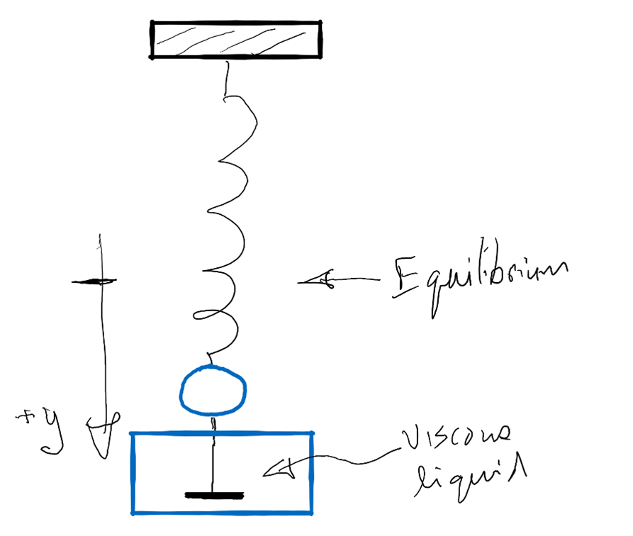
Assume that the spring force is given by Hooke’s law.
\[F_s = - ky\left(t\right)\]
Assume that the damping force is proportional to the object’s velocity.
\[F_d = - cv_y\]
You can ignore the gravitational force for this analysis. Use the following values for the model parameters.
\[\begin{array}{l} m = 0\ldotp 150\left[\text{kg}\right] \\ k = 40\ldotp 0\left[\text{N/m}\right] \\ c = 1\ldotp 50\left[\text{Ns/m}\right] \end{array}\]
For the initial conditions, assume that the spring is stretched 15 [cm] and released from rest. This gives
\[\begin{array}{cc} & y\left(0\right) = 0.15\left[\text{m}\right] \\ & v_y\left(0\right) = 0.0\left[\text{m/s}\right] \end{array}\]
You should use Newton’s second law to find the differential equation for the object’s acceleration. Convert the 2nd order differential equation into two first-order equations. Perform a numerical solution of the two-state variable model. Create a plot of the object’s position as a function of time for \(0 \leq t \leq 1.5\left[\text{s}\right]\). Properly label the graph.
2. The SZR model introduced in Chapter 8 for modeling the zombie infection suggested that humans would always lose the battle and essentially become extinct. Zombie stories often will offer a little more hope for human survival. Can we create another model that might include this possibility? Munz, et al. say yes. They introduce another compartment, the infected population, I, and also allow that zombies can be cured of their disease. They hypothesize the following rate equations for the four compartments:
\[\begin{array}{l} \frac{dS}{dt} = P- bSZ- dS + cZ \\ \\ \frac{dI}{dt} = bSZ- \rho I- dI \\ \\ \frac{dZ}{dt} = \rho I + rR- aSZ- cZ \\ \\ \frac{dR}{dt} = dS + dI + aSZ- rR \end{array}\]
Develop a program that performs a numerical solution of this revised model, which we will call the SIZR model. Since the model has seven parameters \((P, b, d, c, \rho, r, c)\), exploring its behavior is complicated. Start with a set of model parameters that are close to those used in the SZRmodel.py code shown in Figure 10. Assume that there is no cure so that c=0. The initial set of model parameters are
\[P = 0.1\text{ , }b = 9.5e - 3\text{ , }d = 1.e - 4\text{ , }c = 0\text{ , }\rho = 3.0e - 1\text{ , }a = 5.0e - 3\text{ , }r = 1.0e - 4\]
The initial conditions are
\[S\left(0\right) = 100\text{ , }I\left(0\right) = 0\text{ , }Z\left(0\right) =0.1 \text{ , }R\left(0\right) = 0\]
You should find that humans, the S compartment, still get wiped out, but introducing the I compartment delays the time required. Next, explore the effect of a nonzero c parameter value. A good range to explore is \(0 \leq c \leq 0.015\). Calculate the compartment populations for \(0 \leq t \leq 100\).
Write an essay that describes the four steps in our problem-solving strategy. In the Analysis section, provide a figure that illustrates the relationships between the four compartments implied by the rate equations given above.
References
Centers for Disease Control and Prevention (U.S.) & Office of Public Health Preparedness and Response. (2011). Preparedness 101; zombie pandemic. https://stacks.cdc.gov/view/cdc/6023
Edelstein-Keshet, L. (2005). Mathematical Models in Biology. Society for Industrial and Applied Mathematics. https://doi.org/10.1137/1.9780898719147
Kay, G., & Brugués, A. (2012). Zombie Movies: The Ultimate Guide (Second Edition, Second edition). Chicago Review Press.
Munz, P., Hudea, I., Imad, J., & Smith, H. L. (2009). WHEN ZOMBIES ATTACK!: MATHEMATICAL MODELLING OF AN OUTBREAK OF ZOMBIE INFECTION. In J. M. Tchuenche & C. Chiyaka (Eds.), Infectious Disease Modelling Research Progress (pp. 133–150).
Robinson, J. A., Trulear, M. G., & Characklis, W. G. (1984). Cellular reporoduction and extracellular polymer formation by Pseudomonas aeruginosa in continuous culture. Biotechnology and Bioengineering, 26(12), 1409–1417. https://doi.org/10.1002/bit.260261203
Wikipedia Contributors. (2022). List of zombie films. In Wikipedia. https://en.wikipedia.org/w/index.php?title=List_of_zombie_films&oldid=1104193295